Teaching Mathematical Modeling in the
Department of Mathematics
Universitas Padjadjaran
1
Asep K. Supriatna
Department of Mathematics, Universitas Padjadjaran Email: [email protected]
Abstract
In this talk I will present my experience in teaching mathematical modeling in the Department of Mathematics Universitas Padjadjaran. The talk will include the materials that have been taught; the way the materials were presented; and the way the testing were done. In general, there are many aspects, both materially and methodologically, that need some improvement in teaching mathematical modeling in the department. I hope that there will be some insight on how to improve this teaching process from the discussion in this mini-symposium.
1 Presented in the Mini-Symposium on Teaching Mathematical Modelling. International Conference on Applied Mathematics (ICAM05) in Bandung, August 22-26, 2005
What are the details of the subject?
Title: Mathematical Modeling
Code: D1A303 (compulsory)
Level: Year 3
Credit: 4 SCU
Syllabus: Mathematical model and the principles of modeling; Stages in a modeling process; Categories of mathematical models: continuous & discrete models, deterministic & stochastic models, descriptive, predictive & prescriptive models, etc. Brief Description: This subject discusses topics in the application of mathematics.
This is a “problem based” lecture. Some problems from various branches of science and engineering, including physical sciences, life sciences, economics and others are taken and converted into mathematical models (numbers, variables, equations, graphs, etc), we analysis the models using appropriate methods of mathematics to obtain the solutions, and then we interpret the solutions in terms of the original problems where they came from.
Aims: To foster students’ appreciation in mathematics
To encourage students to translate a relatively unstructured problem into an appropriate form to facilitate the solutions To develop students’ skill in communicating mathematical ideas
Learning objective: By the end of the course students be able to:
• understand the process of the formulation, solution, interpretation and evaluation of mathematical models • select an appropriate mathematical methods to obtain the
solution of some sorts of problems
• communicate the solution in a written and oral presentation
Lecturers: Asep K. Supriatna & F. Sukono
Book(s): Walter J. Meyer (1985). Concepts of Mathematical Modeling. McGraw-Hill.
Related subjects:
Mathematical Population Theory (elective)
Why the aims are like so?
Until recently, the only major gate for student to come to universities is by undertaking SPMB (a test for entering an Indonesian state university). In SPMB, students may have two departments as their choice, by specifying the first and the second choice. Once they passed the test, they assigned to one department, depending on their test result. Most students enrolling in the Department of Mathematics Universitas Padjadjaran are those whose mathematics as their second choice in their SPMB. Informal finding revealed that most of them do not know what is mathematics and what is it for in daily life, except that the knowledge of mathematics as a science of number and counting. So, it is not surprising that if they have less appreciation into mathematics. They choose mathematics as their second choice just because their school mathematics is good. State universities is still more prestigious than most private universities, regardless what department they chosen. Most of them have medical, engineering and other favorite departments as their first choice. Many of them are trying to undertake SPMB in the next year. Once they accepted by their favorite department, they left Mathematics Department, for good.
This example shows the importance of giving the knowledge of the application of mathematics in daily life or in other aspects of life as soon as possible for nurturing students’ appreciation in mathematics. This is why we formulate A1 as the first aim in teaching mathematical modeling, and this is why we move mathematical modeling course from level 4 to level 3. Once the students know that mathematics have broad applications in daily life or in other branches of scientific knowledge, it is naturally if we want to arm the students with the knowledge on how to tackle a problem mathematically. Hence, the second aim we formulate is clear by itself. Communication skill is among the goals of education in Indonesia. We comply to this goal by explicitly mention this goal as the third aim in teaching mathematical modeling, with emphasizing in communicating mathematical ideas.
How many students were enrolling this subject? Students:
Year Number of Students
2001 90 (two classes)
2002 108 (two classes)
2003 82 (two classes)
2004 73 (two classes)
2005 Approx. 80 (one class, year
4)
And approx. 80 (one class, year 3)
What are the teaching & learning strategies we used?
There were 32 class-meeting in one semester (including mid semester test and end of semester test). In the first half semester there are twice lectures a week and each has two hours duration. The first fifteen lectures are done by delivering materials taken from a textbook. We present the principles of modeling and give various examples of the modeling process. We use mainly the book written by Meyer (Concepts of Mathematical Modeling). Almost all of the materials for the fifteen lectures are drawn from this book. This includes gravitation models, population growth models, and economics models, in discrete and continuous forms. Usually in the first lecture we discuss the importance and the benefits of modeling in real life or seeing a portion of movie related to modeling, such as Mr. Bond’s movie “The man with the golden gun”, just to motivate the students.
All the problems discussed in the class follow the modeling process described in Meyer’s book as follows:
1. Formulation a. Stating the question
b. Identifying and choosing relevant factors (making a simplification) c. Finding relationship between the relevant factors (making an assumption) d. Converting the relationship into mathematical description (making a model) 2. Mathematical Manipulation
a. Finding a mathematical solution of the resulting model using mathematical tools (calculation, solving an equation, proving theorem, etc.)
3. Evaluation
a. Interpreting the mathematical solution in terms of the original problems b. Questioning the results: such as the correctness of the solution, the accuracy of
the solution, etc.
c. Deciding whether we are satisfied with the results or not 4. Reformulation (if any)
5. Applying the model (in terms of descriptive model, predictive model, or prescriptive model)
How tests are done?
What problems were we encountered?
• The difficulty to find a “real” problem suits to undergraduate students.
In general it was difficult to choose realistic problems that can be solved by third year students. That is why most of the exercises and assignment are taken from published work, such as books and journals to ensure that they have solutions. Most of the “real” problems given to them remain unsolved.
• The reluctant of students to initiate discussion regarding the problem they had. Although we give an opportunity for students to see us to discuss what ever problems that students found in doing they modeling exercises or assignment, there were almost no students come to see.
• The limited resources of books and journals in the department’s library
The collection in our library is very limited. It is often happen that students found a model in which there is no book in our library that contains mathematical method suits to analyze the model. To assist the students we composed a lecture note (diktat) in which inside the diktat there are several pages describing what book are available in what library (department’s, faculty’s, university’s libraries, and even other universities’ libraries), including their call-numbers or Dewey classification call-numbers.
What else?
This semester I will teach modeling for approximately 160 students, due to two reasons: first, the overlapping between new curriculum and the old curriculum, so we have to serve to two levels (3 & 4). Second, about 1/3 of the lecturers are on leave to undertake postgraduate study, so that they could not teach during their study period. I hope there will be no much trouble in handling this huge class.
What were goods?
• More and more students know that mathematics does useful, both in daily life and in many branches of science and technology. Even my own student, who come to our department with mathematics as her second choice in SPMB said, that at the time she was very confident not to move out from this department. Indeed, she undertook SPMB again, and she succeed, just to prove that she could be accepted by her first choice department (architecture in a prestigious institute), but she didn’t take that ticket. Now she is happy doing her job in one of the prestigious bank company applying her mathematical knowledge. • Sometimes we find that what were discussed in modeling class a little bit
“worthy publication”. In this case we could make joint publication with our former modeling students, even though only in a local journal.
Appendix I: Example of Modeling Assignment Manufacturing Progress Curve
Here is the excerpt from Meyer book page 18:
“If you have a complicated job to do and you have to do it many times, you’ll probably get better at it. Partly this matter of learning: practice does make perfect. But ingenuity will also play a role: you will invent shortcuts, devise new tools to assist you, etc. The same is true for a team of workers and managers assembling complex products, like airplanes or automobiles. T.P. Wright studied this in aircraft assembly plants in 1936 and proposed the following model. Since then, it has been used in many branches of manufacturing”.
Wright assumed that when the number of planes is doubled, the time for production decreases to about b%. Wright ended up to the following equation
α
x T x
T()= (1) with α=log2a and a=1−b/100.
The equation is often refereed as a manufacturing progress curve.
1. Read through the Illustration 2 (page 18-20 in Meyer book) carefully. Criticize the model above. Explain why the model proposed by Conway and Schultz is better than the above equation.
2. Browse the internet, find an article on manufacturing progress curve. Make a summary about the article and discuss and compare the model therein to Wright’s model.
Appendix II: Example of Lecturer’s solution to problem 3 (In Indonesian).
Konstruksi Persamaan Perbaikan Produksi Melalui Sistem Dinamis
Abstract
In this paper we discuss a learning curve or manufacturing progress curve of an industrial process. An equation describing this process will be derived by solving a modified logistic differential equation. This derivation is slightly different to that usually done in many industrial engineering literatures. It is shown that the solution to this modified equation satisfies all properties needed by a manufacturing learning curve.
Pendahuluan
Dalam berbagai bidang industri dikenal sebuah fenomena dimana apabila jumlah suatu produk berlipat, maka rata-rata waktu yang diperlukan untuk membuat per satuan produk tersebut berkurang. Hal ini salah satunya dikarenakan adanya proses pembelajaran, yang berakibat dengan berjalannya waktu maka berbagai faktor yang menghambat proses produksi pada industri tersebut dapat diatasi. Istilah lain yang banyak dipakai untuk menggambarkan fenomena ini adalah "learning curve", "experience curve", "learning by doing" atau "learning by use" (Argote dkk, 1990). Dampak pembelajaran tersebut untuk pertama kalinya, secara matematis dipelajari oleh Wright (1936) dengan mempelajari berbagai faktor yang dapat mempengaruhi biaya pembuatan pesawat terbang. Dalam paper ini akan dibahas ulang model Wright tersebut. Selain itu juga akan dibahas sebuah pendekatan alternatif.
Alternatif lain yang eqivalen untuk menggambarkan performance produksi adalah dengan menggambarkan grafik jumlah kesalahan atau biaya per unit produk terhadap waktu atau jumlah produk, yang secara teoritis akan mempunyai bentuk yang sama dengan grafik waktu produksi per unit produk terhadap banyaknya produk. Melalui pendekatan sistem dinamis, yakni dengan melihat laju perubahan kesalahan produksi, dalam paper ini akan dibuat suatu model yang dapat menggambarkan apakah terjadi pembelajaran (perbaikan produksi) atau tidak dalam suatu proses produksi.
Model Kurva Perbaikan Produksi Wright
Pengamatan yang dilakukan Wright (1936) memperlihatkan bahwa biaya yang diperlukan untuk membuat sebuah pesawat terbang berkurang sebesar 20% setiap produksi berlipat dua dari sebelumnya. Dalam model yang dikembangkannya, Wright berasumsi bahwa “apabila jumlah suatu produk berlipat dua, maka rata-rata waktu yang diperlukan untuk membuat per satuan produk tersebut berkurang sebesar b%”. Dari asumsi tersebut dapat diturunkan pernyataan-pernyataan matematis berikut.
Misalkan T(n) adalah waktu yang diperlukan untuk membuat produk ke-n. Dari asumsi tersebut dapat disimpulkan bahwa waktu yang diperlukan untuk menghasilkan produk ke i=2n,
(n=0,1,2,3, …) adalah
n n
a T
T(2)= (1) , 1
dengan a=1-b/100. Rumus tersebut hanya berlaku untuk bilangan yang merupakan perpangkatan dari 2. Untuk memperumum rumus di atas, maka persamaan tersebut diubah ke dalam bentuk
Dengan mengambil logaritmanya maka diperoleh
a
x T
a x T
x
T log2
2 2
2 2 2
2 ( ) log ( (1)) log log log ( (1)) log
log = + = +
) ) 1 ( ( log ) (
log2 2
α
x T x
T =
atau
α
x T x
T( )= (1) 3
dengan α=log2a. Persamaan terakhir ini dinamakan persamaan perbaikan produksi yang juga
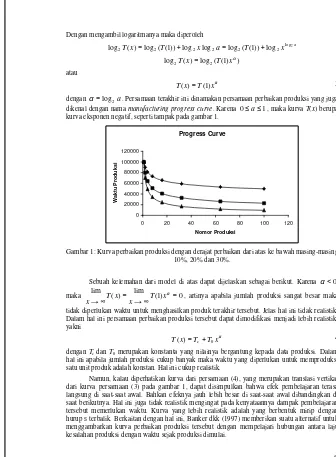
dikenal dengan nama manufacturing progress curve. Karena 0≤a≤1, maka kurva T(x) berupa kurva eksponen negatif, seperti tampak pada gambar 1.
Progress Curve
0 20000 40000 60000 80000 100000 120000
0 20 40 60 80 100 120
Nomor Produksi
Waktu Produksi
Gambar 1: Kurva perbaikan produksi dengan derajat perbaikan dari atas ke bawah masing-masing 10%, 20% dan 30%.
Sebuah kelemahan dari model di atas dapat dijelaskan sebagai berikut. Karena α<0
maka lim ( ) lim (1) =0
∞ → = ∞
→ T x x T xα
x , artinya apabila jumlah produksi sangat besar maka
tidak diperlukan waktu untuk menghasilkan produk terakhir tersebut. Jelas hal ini tidak realistik. Dalam hal ini persamaan perbaikan produksi tersebut dapat dimodifikasi menjadi lebih realistik, yakni
α
x T T x
T()= c+ 0 4
dengan Tcdan T0 merupakan konstanta yang nilainya bergantung kepada data produksi. Dalam
hal ini apabila jumlah produksi cukup banyak maka waktu yang diperlukan untuk memproduksi satu unit produk adalah konstan. Hal ini cukup realistik.
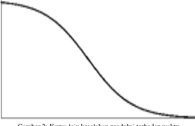
Model Laju Kesalahan Produksi Banker
Misalkan x=f(t) menunjukkan jumlah kesalahan produksi pada saat t. Grafik yang diharapkan dari x terhadap t adalah seperti pada gambar 2 berikut.
Gambar 2: Kurva laju kesalahan produksi terhadap waktu
Kurva seperti pada Gambar 2 dapat diperoleh apabila dx/dt<0 untuk setiap saat t. Selain itu nilai absolut dari dx/dt membesar secara perlahan pada saat awal, kemudian semakin membesar dengan kecepatan perubahan yang membesar dan mencapai puncak di titik infleksi tinf. Setelah itu nilai absolut dx/dt tersebut mengecil. Secara matematis, syarat cukup agar diperoleh kondisi di atas adalah
t dt
dx
∀
≤0, 5
inf 2
2
,
0 t t
dt x d
<
≤ 6
inf 2
2
,
0 t t
dt x d
=
= 7
inf 2
2
,
0 t t
dt x d
>
≥ 8
t dt
x d
∀ ≥0,
3
3 9
Persamaan (5)-(9) dapat dipakai sebagai kriteria untuk menentukan apakah dalam sebuah proses produksi terjadi pembelajaran atau tidak. Sebagai ilustrasi, misalnya Banker dkk (1997) mempelajari data tentang pengaruh team-work terhadap kualitas produksi dengan melihat
banyaknya kesalahan yang terjadi secara longitudinal. Dari data ini dilakukan regresi polinom derajat 3, yakni
3 2
)
(t t t t
f
x= =α+β +γ +δ 10
Dengan menurunkan x terhadap t akan diperoleh 2
3 2
/dt t t
dx =β+ γ + δ ,
t dt
x
d2 / 2=2γ+6δdan δ
6
/ 3
3 =
dt x
d . Kriteria terjadinya proses pembelajaran dapat ditentukan dengan melihat apakah kondisi (5)-(9) terpenuhi atau tidak, dengan tinf merupakan akar dari persamaan 2 / 2=2 +6 =0
t dt
x
d γ δ , yakni tinf =−γ/3δ.
Penggunaan regresi terhadap polinom derajat 3 yang dilakukan Banker dkk bermanfaat untuk memperoleh model keberhasilan team-work dalam rentang waktu dimana data tersedia, tetapi mungkin tidak dapat diekstrapolasi. Sebuah counter example tentang penggunaan polinom derajat 3 untuk menggambarkan kurva perbaikan produksi akan diberikan oleh contoh hipotetis yang diambil dari Meyer (1984).
Soal no 14 halaman 21 pada buku Meyer meminta model fungsi kemajuan produksi untuk data berikut
Jumlah Produksi 1 2 4 8
Jam Pekerja 32000 25600 20480 16384
Jawaban untuk soal di atas adalah 0,322
32000 )
(x = x−
T dengan laju perbaikan produksi 20%. Akan tetapi apabila soal ini sedikit dimodifikasi, “jam pekerja” diganti dengan “banyaknya kesalahan”, di mana keduanya menggambarkan fenomena yang sama, yakni perbaikan produksi, maka dengan menggunakan regresi polinom derajat 3 (leastsquare, Maple V) diperoleh persamaan Y(x)=294912/7−12288x+2304x2−1024/7x3. Kurva untuk kedua persamaan tersebut terlihat pada gambar 3. Kondisi (5)-(9) yang disyaratkan Banker dkk tidak terpenuhi (contohnya d3x/dt3=−6(1024/7)<0, ∀t
). Bahkan untuk nilai x yang sangat besar Y(x) bernilai negatif, yang sangat tidak realistik. Dalam bagian selanjutnya akan dibahas bagaimana mengkonstruksi suatu persamaan yang memenuhi kondisi (5)-(9) di atas melalui sistem dinamis.
Persamaan Implisit Perbaikan Produksi
Dalam bagian ini perbaikan produksi akan dicirikan oleh penurunan jumlah kesalahan produksi. Kurva perbaikan yang diharapkan, seperti pada gambar 2, mirip dengan solusi persamaan diferensial logistik dx/dt=ax−bx2 yang mempunyai dua solusi setimbang (steady state solution), yakni x=0 yang tidak stabil dan x=a/b yang stabil (Braun, 1982, hal. 29). Solusi lain dengan nilai awal x0 (0<x0<a/b) mempunyai trayektori seperti pada gambar 4c. Dengan ide yang sama kita dapat membuat persamaan diferensial untuk menggambarkan laju perubahan banyaknya kesalahan yang dibuat. Diasumsikan bahwa “dari waktu ke waktu banyaknya kesalahan berkurang dan perubahannya sebanding dengan kesalahan yang sudah dibuat”. Jika x(t) menunjukkan banyaknya kesalahan pada waktu t, maka dinamik dari banyaknya kesalahan tersebut diberikan oleh
ax dt dx
−
= . 11
Karena perubahannya sebanding dengan jumlah kesalahan, maka semakin banyak kesalahan perubahan semakin besar. Hal ini tidak kurang realistik karena tidak memuat faktor kejenuhan yang dapat meredam laju perubahan tersebut. Diasumsikan “bahwa faktor kejenuhan ini sebanding dengan kwadrat jumlah kesalahan”, sehingga dinamik dari jumlah kesalahan tersebut akan berbentuk
) (
2
x f bx ax dt dx
≡ + −
= . 12
Untuk melihat sifat solusi dari persamaan di atas akan dipelajari solusi setimbang (titik tetap) x=0 dan x=a/b yang diperoleh dari kondisi f(x)=0. Kestabilan dapat dilihat dengan memeriksa tanda dari f'(x) di kedua titik ini, yakni f'(0)=−a<0dan f'(a/b)=a>0, yang berarti x=0 stabil dan x=a/b tidak stabil (lihat Hale & Kocak, 1991, hal. 17-18 untuk definisi dan syarat kestabilan). Sehingga kurva solusi untuk nilai awal x0 (0<x0<a/b) seperti pada gambar 4a. Kurva ini terlalu ideal, karena pada akhirnya jumlah kesalahan akan nol. Untuk memperbaikinya kita lakukan langkah berikut.
Dengan mengikuti cara yang sama, kurva yang diinginkan harus merupakan kurva dari persamaan x(t) yang merupakan solusi persamaan diferensial yang mempunyai titik tetap x=c yang stabil dan x=a/b yang tidak stabil. Kedua titik tetap berasal dari persamaan
) ( ) )(
(x c bx a g x
dt dx
≡ − −
= . 13
Kita klaim bahwa x=c stabil dan x=a/b tidak stabil apabila dipenuhi syarat c<a/b. Hal ini dapat dibuktikan sebagai berikut. Turunan pertama dari g(x) adalah g'(x)=2bx−(a+bc), sehingga
0 )
( 2 ) (
'c = bc− a+bc =bc−a<
g apabila c<a/b . Dengan alasan yang sama diperoleh
0 )
( ) / ( 2 ) / (
'a b = ba b − a+bc =a−bc>
g .
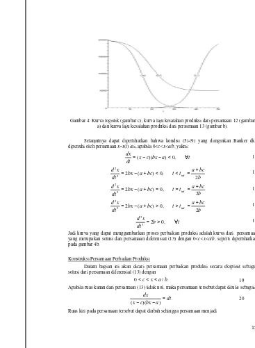
Gambar 4: Kurva logistik (gambar c), kurva laju kesalahan produksi dari persamaan 12 (gambar a) dan kurva laju kesalahan produksi dari persamaan 13 (gambar b).
Selanjutnya dapat diperlihatkan bahwa kondisi (5)-(9) yang diinginkan Banker dkk dipenuhi oleh persamaan x=x(t) ini, apabila 0<c<x<a/b, yakni:
t a
bx c x dt
dx= − − < ∀
, 0 ) )(
( 14
b bc a t t bc a bx dt
x d
2
, 0 ) (
2 inf
2
2 +
= < < + −
= 15
b bc a t t bc a bx dt
x d
2
, 0 ) (
2 inf
2
2 +
= = = + −
= 16
b bc a t t bc a bx dt
x d
2
, 0 ) (
2 inf
2
2 +
= > > + −
= 17
t b dt
x
d = > ∀
, 0 2
3 3
18
Jadi kurva yang dapat menggambarkan proses perbaikan produksi adalah kurva dari persamaan yang merupakan solusi dari persamaan diferensial (13) dengan 0<c<x<a/b, seperti diperlihatkan pada gambar 4b.
Konstruksi Persamaan Perbaikan Produksi
Dalam bagian ini akan dicari persamaan perbaikan produksi secara eksplisit sebagai solusi dari persamaan diferensial (13) dengan
b a x
c /
0< < < . 19
Apabila ruas kanan dari persamaan (13) tidak nol, maka persamaan tersebut dapat ditulis sebagai
dt a bx c x
dx =
−
− )( )
dt a bx
bdx c x
dx a
bc =
− − + − −
1
. 21
Dengan mengintegralkan kedua ruas maka diperoleh
(
ln ln)
11
K t a bx c x a
bc− − − − = + , 22
Dengan K1 merupakan konstanta integrasi. Selanjutnya persamaan ini dapat diubah sebagai berikut:
) )( ( ln ln
ln t K1 bc a
a bx
c x a bx c
x = + −
− − = − −
− , 23
atau
) )( (tK1 bca
e a bx
c
x = + −
−
− . 24
Selanjutnya karena syarat persamaan (19) harus dipenuhi dan dengan memisalkan
a bc
D= − maka diperoleh
) (tK1 D
e bx a
c
x = +
−
− , 25
atau
) ( 1 )
( DtK
e bx a c
x− = − + . 26
Dengan penulisan ulang diperoleh
c ae be
x(1+ D(t+K1))= D(t+K1)+ . 27 Dari persamaan terakhir dapat diperoleh bentuk eksplisit dari x sebagai fungsi dari t, yaitu
2 2 )
( ) (
1 1
1 1
1
1 1
K be
c K ae e be
c e ae be
c ae x
Dt Dt DK Dt DK Dt K t D K t D
+ + = +
+ =
+ +
= +
+
. 28
Konstanta K2 dapat ditentukan dari nilai awal x(0)=x0, yakni
0 0 2
bx a
c x K
− −
= . Perhatikan bahwa
nilai D<0, sehingga xt c t→∞ ()=
lim
. Dengan demikian dapat disimpulkan bahwa persamaan (28)
merupakan persamaan eksplisit yang kita cari sebagai persamaan perbaikan produksi.
Kesimpulan
Dalam paper ini telah dikonstruksi sebuah model yang dapat menggambarkan proses perbaikan produksi yang mengakomodir “learning process” dengan memanfaatkan sifat-sifat sistem dinamis. Dengan menyederhanakan notasi secara umum persamaan perbaikan produksi akan berbentuk
Bt Bt
De C Ae t
x −
− +
+ =
1 )
( , 29
Dengan A, B, C dan D konstanta-konstanta positif.
Referensi:
1. Argote, L., Beckman, S.L. and Epple, D. (1990). The Persistence and Transfer of Learning in Industrial Settings, Management Science Vol. 36 No. 2, pp. 140-154. 2. Banker, R.D, J.M. Field dan K.K. Sinha (1997). Workteam Implementation and
Trajectories of Manufacturing Quality: a Longitudinal Field Study. Internet.
3. Braun, M. (1982). Differential Equations and Theirs Applications. Springer-Verlag, New York.
4. Dutton, J.M. and Thomas, A. (1984). Treating Progress Functions as a Managerial Opportunity, Academy of Management Review Vol. 9 No. 2, pp. 235-247.
5. Hale, J. & H. Kocak (1991). Dynamics and Bifurcations. Springer-Verlag, New York. 6. Meyer, W.J. (1984). Concept of Mathematical Modeling. McGraw-Hill Int. Edn.,
Singapore.
7. Wright, T.P. (1936). Factors Affecting the Cost of Airplanes, Journal of Aeronautical Science Vol. 3, p. 122.
Appendix III: Example of Lecturer’s solution to problem 3.
Parameter Determination in Manufacturing Progress Curve with Three Points of Data
Abstract
In this paper we discus a method to find the values of parameters in a manufacturing progress curve based on three points of data. In general to find better parameter estimation we need a lot of data. However, in some circumstances, the numbers of data are limited or even scarce, especially in the beginning of a manufacturing process. For this reason, we develop a simple method to determine the values of parameters if only three data are available. The curve we are dealing with is an inverse-like sigmoid that can describe a learning process in the beginning phase and has a lower bound in the long-term phase, hence a reasonably realistic curve.
Keywords: Manufacturing progress curve, curve fitting, sigmoid curve.
Introduction
In many industrial or manufacturing processes there is a phenomenon that when the numbers of product multiplies or when the time of production goes on then the average time needed to produce a unit product decreases. Among the reasons is because of the learning process, in which by the time goes on there will be some improvement in the process. A mathematical term to describe this phenomenon is known as a
learning curve or an experience curve (Yelle, 1979; Argote et al., 1990). Wright (1936) was among the first who investigated the effect of this kind of learning in a manufacturing process by studying various factors affecting the cots of aircraft production. This curve is able to describe the performance of the aircraft manufacturing process.
An equivalent alternative to figure out the performance of a manufacturing process is by a curve showing the numbers of production faulty or the per capita cost level as a function of time or the numbers of product. The curve will have a similar form to the curve showing the time needed to produce a unit product against the total numbers of product. If x(t) denotes the numbers of production error in the time of
t, then Supriatna and Husniah (2004) show that the production progress curve can be described by equation
K be c K ae t
x Dtt
t t D ) ( ) ( 0 0 1 ) ( − − + +
= . 1
where a, b and c are positive constants satisfying 0<c<x<x0<a/b, D=bc−a<0. The
constant K can be obtained from the initial value x(t0)=x0, that is
0 0 bx a c x K − −
= . Since D<0 then
c t x t→∞ ()=
lim
, means that eventually the numbers of production faulty is a constant c.
Considering the non-linearity of equation (1), the parameter estimation by regressing known data to that equation is not easy. In this paper we will develop a simple method to determine a, b and c in equation (1) if there are three successive data known.
Determining the value of a/b
Suppose three successive data x(t0),x(t1),x(t2)are known with t1−t0=t2−t1=∆t. We want to determine the curve passing all the data points satisfying equation (1) whenever the value of c is known. To find the values of a and b we first find the value of a/b.
) (t x 1 ) ( ) ( 1 1 1 ) ( 0 1 0 1 x K be c K ae K be c K ae t
x Dt
t D t t D t t D ≡ + + = + + = ∆ ∆ − −
. 2
It can be rewritten in the form of
1 1 1 1 1 − = − ⇒ + = + ∆ ∆ ∆ x c x a b K e x c K ae K
be Dt
t D t D
. 3
Solving for t, we find the following expression
(
bx a)
K x c x a b K x c eDt
− − = − − = ∆ 1 1 1 1 1
. 4
Analogously, for x(t2), we have
(
bx a)
K x c x a b K x c eDt
− − = − − = ∆ 2 2 2 2 2 1
. 5
Next, from (5) and (4), it can be obtained that
(
)
(
)
2 1 1 2 2 − − = − − a bx K x c a bx K x c 6 or(
)(
)
(
)(
)
(
(
) (
) (
)
)
(
(
)
)
(
(
) (
)(
)
)
2 1 0 0 2 1 2 2 2 1 2 0 2 0 2 1 2 0 0 2 a bx c x bx a x c a bx x c a bx c x bx a x c a bx c x bx a x c − − − − = − − ⇒ − − − − = − − − −, 7
which can be rearranged into
(
)(
)
(
)
(
) (
)(
)
2 0 2 1 2 1 02 bx a bx a a bx
x c
c x x
c − = − −
− − −
. 8
Furthermore, if
(
)(
)
(
−)
=λ − − 2 1 0 2 x c c x x c, then equation (8) becomes
(
)
(
)
0 22 2 0 2 2 1 2 1 2
2abx a abx x a bxx
x
b − + = + − −
λ . 9
which can be simplified into
(
)
(
2)
2(1 ) 00 2 1 2 0 2 1
2λ + − λ + + + +λ =
a x x x ab x x x
b . 10
(
)
(
2)
(1 ) 02 0 2 1 2 0 2
1 + =
+ + + − + λ λ λ b a x x x b a x x
x . 11
Consequently
b a
R
x b a=
. 12
Determining the values of a and b
The following procedure is done to find the explicit forms of a and b. Note that equation (2) can be written in the forms of
(
) (
)
(
)
e(
x c)
x a bx a bx a c c x ae bx a c x e x a c bx a c x ae K e x a c K ae K be c K ae x t D R t D t D R t D t D R t D t D t D − + − − + − = − − + + − − = + + = + + = ∆ ∆ ∆ ∆ ∆ ∆ ∆ ∆ 0 0 0 0 0 0 0 0 1 1 1 1 .
(
0)
(
0)
(
0) (
0)
1 e x c ae x c ca bx
x a bx a
x Dt Dt
R − + − =
− + ∆ − ∆ . 13
(
)
=(
−)
+ − + − − ∆ ∆ 0 0 0 0 1 x x a a c c x ae c x e x a x x a a x R t D t D R R. 14
The two sides of this equation are divided by aand changed into
(
)
− − − = − − ∆ 0 1 1 0 01 1 1 1 x
x x x x x c c x x x e R R R t D
. 15
(
) (
= −)
− − − ∆ 0 1 0 1 1 1 1 x x x c c x x x e R R t D. 16
(
)
(
)
(
)
(
−)
− − − = − − − − = ∆ R R R R t D x x x c x x x c c x x x x x x c e 1 0 0 1 0 1 0 1 1 1 1 1 1. 17
Hence
(
)
(
−)
− − − = ∆ R R x x x c x x x c t D 1 0 0 1 1 1ln or
(
)
(
−)
− − − = ∆ − R R x x x c x x x c t a bc 1 0 0 1 1 1 ln )( , and finally we obtain
(
)
(
−)
− − − = ∆ − R R R x x x c x x x c t a c x a 1 0 0 1 1 1ln . The last equation gives the explicit form of a, that is
(
)
(
−)
− − − ∆ − = R R R x x x c x x x c t x c a 1 0 0 1 1 1 ln 1 1. 18
The explicit form of b can be obtained straight away, that is
R
x a
b= 19
In this case xRis given by equation (12) as the positive root of (11).
A Numerical Example
In this section we provide a numerical example to illustrate the method. Suppose three data measuring the numbers of faulty product at times t=0, t=25 and t=50 are known. They are x(0)=19800,
8200 ) 25
( =
x and x(50)=5050. It is clear that the time intervals are uniform, that is 1
2 0
1 t 25 0 25 50 25 t t
t
t= − = − = = − = −
∆ . Furthermore it is also known that the lower bound of the numbers of product is c=5000. Solving equation (11) and (12), we find
21053 . 20508
= =xR
b a
Figure 1
The curve of the manufacturing progress equation (1) with the values of parameters from equations (11), (12), (18) and (19). All the three data points lie exactly on the curve.
Concluding Remark
In this paper we have developed a simple method to obtain a manufacturing progress curve based on three known points of data. This method gives a very good solution, that the resulting curve exactly passes all the three data. However, to use the method described in this paper we need to know the lower bound value c. In practice, this value is might be difficult to obtain in the beginning phase of a manufacturing process. It suggests a future direction of a further investigation. We need a method that free from this additional requirement.
References:
1. Argote, L., Beckman, S.L. and Epple, D. (1990). The Persistence and Transfer of Learning in Industrial Settings, Management Science Vol. 36 No. 2, pp. 140-154.
2. Husniah H. and A.K. Supriatna (2004). The Construction of a Manufacturing Progress Curve Through a Dynamic System. Integrative Mathematics Vol. 3.
3. Wright, T.P. (1936). Factors Affecting the Cost of Airplanes, Journal of Aeronautical Science Vol. 3, p. 122.
4. Yelle, L.E. (1979). The Learning Curve: Historical Review and Comprehensive Survey, Decision Sciences Vol. 10, pp. 302 – 328.
Appendix:
The Derivation of Equation (1)
dx
=
The LHS of the equation is re-arranged and both sides are then integrated as follows.
∫
∫
∫
=
− − + − −
t
t x
x x
x
dt a bx
bdx c x
dx a bc
0
0 0
1
.
The integration yields:
0 0
0
ln ln
1
t t a bx
a bx c x
c x a
bc = −
− − − − −
− ,
(
)(
)
(
)(
)
( )( )ln 0
0
0 t t bc a
a bx c x
a bx c x
− − = − −
− −
,
(
)(
)
(
0)(
)
( )( )0 ett0 bca
a bx c x
a bx c
x − −
= − −
− −
.
(
)(
) (
)(
)
( )( )0 0
0 bca t t
e a bx c x a bx c
x− − = − − − −
(
) (
(
)
)(
)
( )( )0
0 bx aett0 bca
a bx
c x c
x − − −
− − = −
(
)
(
)
(
(
0)
)
( )( )0
0
0 0
1 tt bca
e a bx
c x a c a bx
c x b
x − −
− − − =
− − −
(
)
(
)
(
)
(
)
1) (
0 0
) )( (
0
0 0
+ −
− + −
− = ≡
− −
bx a
c x b
c e
bx a
c x a t x x
a bc t t