TOWARDS CONSISTENT MAPPING OF URBAN STRUCTURES – GLOBAL HUMAN
SETTLEMENT LAYER AND LOCAL CLIMATE ZONES
B. Bechtel a,*, M. Pesaresi b, L. See c, G. Mills d, J. Ching e, P.J. Alexander f, J.J. Feddema g, A.J. Florczyk b, I. Stewart h
a
University of Hamburg, Center for Earth System Research and Sustainability, Hamburg, Germany.
*
b
European Commission, Joint Research Centre (JRC), Institute for Protection and Security of the Citizens (IPSC), Global Security and Crisis Management Unit, Italy
c International Institute for Applied Systems Analysis, Laxenburg, Austria d
University College Dublin, Ireland
e
Institute for the Environment at UNC, Chapel Hill, NC, USA
f
Maynooth University, Ireland
g
University of Victoria, Department of Geography, Canada
h
Univ. of Toronto, Dept. of Civil Engineering, Canada
Commission VIII, Special Session SpS 17
KEY WORDS: Local Climate Zones, Global Human Settlement Layer, LULC, Urban Structure, Urban Systems.
ABSTRACT:
Although more than half of the Earth’s population live in urban areas, we know remarkably little about most cities and what we do know is incomplete (lack of coverage) and inconsistent (varying definitions and scale). While there have been considerable advances in the derivation of a global urban mask using satellite information, the complexity of urban structures, the heterogeneity of materials, and the multiplicity of spectral properties have impeded the derivation of universal urban structural types (UST). Further, the variety of UST typologies severely limits the comparability of such studies and although a common and generic description of urban structures is an essential requirement for the universal mapping of urban structures, such a standard scheme is still lacking. More recently, there have been two developments in urban mapping that have the potential for providing a standard approach: the Local Climate Zone (LCZ) scheme (used by the World Urban Database and Access Portal Tools project) and the Global Human Settlement Layer (GHSL) methodology by JRC. In this paper the LCZ scheme and the GHSL LABEL product were compared for selected cities. The comparison between both datasets revealed a good agreement at city and coarse scale, while the contingency at pixel scale was limited due to the mismatch in grid resolution and typology. At a 1 km scale, built-up as well as open and compact classes showed very good agreement in terms of correlation coefficient and mean absolute distance, spatial pattern, and radial distribution as a function of distance from town, which indicates that a decomposition relevant for modelling applications could be derived from both. On the other hand, specific problems were found for both datasets, which are discussed along with their general advantages and disadvantages as a standard for UST classification in urban remote sensing.
*
Corresponding author
1. INTRODUCTION
The urban effect on the local environment has been the subject of study for more than 150 years. The urban fabric, i.e. the replacement of natural cover with impermeable paving, manufactured materials with specific hydrophobic, thermal and radiative properties, along with the urban form and function, i.e. the dimensions and placement of buildings and energy use, serves to modify the local hydrology and thermal climate in particular. In addition, the fluxes of materials, energy, water and so on that arise from human activities result in the production of wastes that degrades air (pollutants, GHGs), water and soil quality. Taken together, the accumulated decisions on city form and function have a profound and lasting environmental impact.
Until recently, these urban effects were largely seen as a local-scale issue that are best studied and responded to at that local-scale. Sustained and accelerating global urbanisation and the recognition of the impact of cities on global climate change (and vice versa) have changed this view. Moreover,
improvements in atmospheric modelling capacity now permits multi-scalar approaches that can incorporate urban scale processes into global climate models (Jackson et al., 2010). These developments are central to the creation of a global urban climate science that can simulate urban trajectories and provide projections to support mitigation and adaptation policies. However, a major obstacle to progress is the absence of useful global data on urban landscapes; this gap is recognised in the latest IPCC assessment reports on both adaptation and mitigation (Pachauri et al., 2014). These data should capture details on the intra-urban landscape using a consistent approach that yields appropriate data in a timely fashion.
Currently, most of the available global databases provide the urban mask, i.e., the boundaries separating the urban from the ‘natural’ landscape (Esch et al., 2013). These databases, which are created from available satellite data, are often supplemented with population data to yield varying estimates of the global urban footprint. However, these footprints need to be spatially decomposed into universal urban structural types (UST) to be useful for climate studies. Ideally, these data on urban form The International Archives of the Photogrammetry, Remote Sensing and Spatial Information Sciences, Volume XLI-B8, 2016
would be complemented by information on aspects of urban function (e.g. traffic, building energy use, etc.). With regard to the derivation of a global database on UST, the complexity of urban built forms, the heterogeneity of materials, and the multiplicity of spectral properties has impeded progress using the available satellite information. UST studies to date have focussed on only individual cities where the data used are not generic enough to be applied on a global basis (Heiden et al., 2012; Voltersen et al., 2015).
There are a number of UST typologies that have been developed for specific cities but a common and generic typology is a necessary attribute for universal mapping. Recently, there have been two developments in urban mapping that have the potential for providing a standard approach: the World Urban Database and Portal Tools (WUDAPT) and the Global Human Settlement Layer (GHSL) methodology. WUDAPT employs the Local Climate Zone (LCZ) classification scheme (Stewart and Oke, 2012), available satellite data and local expertise to describe the characteristics of different urban neighbourhoods in a city landscape (Bechtel et al., 2015). The GHSL methodology, designed for fully automatic production of built-up density maps, integrates several available sources that characterize global human settlement phenomena, and remotely sensed imagery. In addition, it delivers an experimental GHSL LABEL product that gathers built-up areas characteristics stratified by vegetation cover and building height (Pesaresi et al., 2016a). In this paper the WUDAPT-LCZ scheme and the GHSL LABEL product are compared based on selected cities and their advantages and disadvantages as a standard for UST classification in urban remote sensing are discussed.
2. DATA AND METHODS
2.1 Global Human Settlement Layer
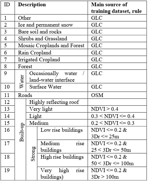
The GHSL methodology, which has been developed and maintained by the Joint Research Centre (JRC), provides a new way to map, analyze, and monitor settlements and urbanization. It is a fully automatic procedure in which the image information extraction workflow processes multi-resolution (0.5 m-75 m), multi-platform (e.g., SPOT, Landsat, Sentinel), multi-sensor (pan, multispectral), and multi-temporal image data successfully (Pesaresi et al., 2013). For example, the European Settlement Map 2014 (http://land.copernicus.eu/pan-european/GHSL/) is based on SPOT5-6 satellite imagery. Recently, the GHSL methodology has been used to produce a new global information baseline describing the spatial evolution of the human settlements in the past 40 years (Pesaresi et al., 2016a). The information has been extracted from Landsat image records organized in four collections, i.e. the epochs 1975, 1990, 2000, and 2014. The core processing methodology relies on a new supervised classification paradigm developed for real big remote sensing data scenarios (Pesaresi et al., 2016b). The main products delivered at 38m resolution (in Google Mercator projection) are: an estimation of the global built-up area per epoch, and an experimental GHSL LABEL product that extends GHSL classification schema to multiple-class land-cover. The GHSL LABEL dataset (Table 1), in short LABEL, has been produced from the epoch 2014 collection. The not built-up areas are discriminated using Meris Globcover (GLC) (Bontemps et al., 2011) and OpenStreetMap (www.openstreetmap.org) (OSM). The built-up areas are discriminated using several training sets, e.g. MODIS (Schneider et al., 2009) and Landscan (http://web.ornl.gov/sci/landscan/), and further reclassified
using vegetation contents (NDVI) and volume of buildings (3Dr), the latter estimated from integration of SRTM (www2.jpl.nasa.gov/srtm/) and ASTER-GDEM (gdem.ersdac.jspacesystems.or.jp/) data. The class 12 (highly reflecting roof) is made by intersection of built-up areas (detected by GHSL workflow) and pixels classified as cirrus clouds in the Landsat 8 imagery (band 9). The USGS algorithm, which produces the band 9, is known from false positives in highly reflecting materials (e.g. dry soils, silicosis rocks and large concrete roofs), and modern, large prefabricated buildings (such as commercial buildings) fit these criteria. Therefore, the class 12 can be associated to productive and commercial use.
ID Description Main source of
training dataset, rule
1 Other GLC
2 Ice and permanent snow GLC 3 Bare soil and rocks GLC 4 Shrubs and Grassland GLC 5 Mosaic Croplands and Forest GLC
6 Rain Cropland GLC
7 Irrigated Cropland GLC
8 Forest GLC
Highly reflecting roof
13 Very light NDVI > 0.4
Table 1. Classes of the GHSL LABEL product, the main source used to derive training datasets, and thresholds used in built-up area classification.
2.2 Local Climate Zones Mapping
The LCZ classification scheme arose in the absence of a standardised approach for describing and reporting on meteorological field sites commonly used in UHI studies (Stewart, 2011). The scheme employs characteristics that yield the greatest impact on the local scale thermal climate within cities during synoptic conditions, conducive to strong UHI development. As a result, LCZs provide a much needed context for intra-urban variations in observed nocturnal air temperature (Stewart and Oke, 2012). LCZs offer a more purposeful description of measurement sites than the traditional urban-rural dichotomy, and their use is analogous to the attempts to move beyond the derivation of urban masks towards detailed internal discretisation of urban land cover.
The subsequent uptake and application of the LCZ scheme is likely due to the level of information that informs each of its zone types. The basic classification scheme is comprised of 10 urban and 7 non-urban zones – see Table 2. Each of the urban zones are derived from readily recognisable combinations of particular urban forms, functions, cover, fabric and metabolism, The International Archives of the Photogrammetry, Remote Sensing and Spatial Information Sciences, Volume XLI-B8, 2016
which might surround an urban measurement site and yield a distinctive impact on the near surface climate. Since LCZs refer to regions of uniform urban cover, morphology, materials and human activity, and furthermore describe these characteristics in a standardised manner, it is not surprising that the utility of LCZs for applications beyond the description of measurement sites, e.g. for modelling (Alexander et al., 2015; Ching, 2013) or mapping (Bechtel et al., 2015), has been suggested, and that mapping LCZs across an urban area is a worthwhile endeavour. Multiple schemes for mapping LCZs have been suggested and evaluated in the course of developing the WUDAPT project, including: (i) manual sampling of individual grid cells using a Geo-Wiki and subsequent digitisation of homogenous LCZs; (ii) a GIS-based approach using building data (Lelovics et al., 2014); (iii) object-based image analysis (Gamba et al., 2012); and (iv) supervised pixel-based classification (Bechtel and Daneke, 2012). To achieve the aims of universality and transferability demanded by WUDAPT, (iv) was found to be comparably robust and largely objective compared with other mapping schemes (Bechtel et al., 2015).
However, when mapping LCZs utilizing remote sensing data, it has been noted that a particular urban LCZ type will exhibit different spectral properties in different parts of the world, which arise as a result of differing cultural construction practices, materials and background climate (Schneider et al., 2009). Therefore, examples of each class for each city are needed to train the classifier with the respective spectral signatures. This makes local knowledge of the urban structures (along with familiarity with training samples and the LCZ scheme) a critical component of the mapping process. Different data sources have also been considered and eventually multi-spectral and thermal Landsat data from different seasons were chosen, which implies that the discrimination is based on urban cover and fabric rather than structure and metabolism. Nevertheless, LCZ maps have been produced for multiple cities using the non-proprietary software packages Google Earth and SAGA GIS (Conrad et al., 2015), as highlighted in Figure 1.
ID Zone Name ID Zone Name ID Zone Name
1 Compact highrise 4 Open highrise 8 Large lowrise
2 Compact midrise 5 Open midrise 9 Sparsely built
3 Compact lowrise 6 Open lowrise 10 Heavy industry
7
Table 2. Classes of the Local Climate Zones scheme.
An overview of the cities and classifications selected for this study are given in Figure 2. The classifications from Lisboa, Beijing, Chicago, Sao Paulo, Milan and Hong Kong are from the WUDAPT database (March 2016), the Khartoum
classification is from (Bechtel et al., 2016) (training version 6, all features) and Madrid is from (Brousse et al., 2016).
2.3 Colour maps for visual comparison
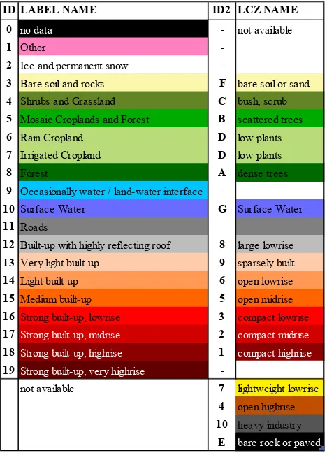
A direct comparison of the two classification schemes is difficult, since the classes cannot be harmonized in a straightforward way. Therefore, in this paper, a visual comparison was undertaken as a first step. To achieve this, a colour coding was developed that aims to display similar classes in the same colours. This assignment was done based on the descriptions and general characteristics of the classes, while it is clear that the same colours do not mean class identity. The common colour scheme is presented in Table 3.
3. RESULTS
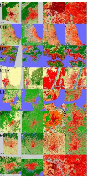
The classifications maps for the selected cities are provided in Figure 2. Largely, the built-up structures agree, while the internal structuring differs. Generally, LABEL preserves more detail due to the higher grid resolution while for the LCZ, the internal structure seems clearer (e.g. for Milan and Sao Paulo). The accordance between both datasets differs. This might be due to random proximity of the used Landsat features or the unlike biophysical backgrounds which affect the supervised LCZ classification and fixed thresholds differently. Since the direct visual comparison is limited, Milan with its surrounding area was selected as a test case for further comparison due to its diversity in landscapes and interesting structure with old village cores in the North and planned development in the South. For this test case, contingency and the accordance of class subsets on a coarser grid were evaluated.
ID LABEL NAME ID2 LCZ NAME
0 no data - not available
1 Other
-2 Ice and permanent snow
-3 Bare soil and rocks F bare soil or sand
4 Shrubs and Grassland C bush, scrub
5 Mosaic Croplands and Forest B scattered trees
6 Rain Cropland D low plants
7 Irrigated Cropland D low plants
8 Forest A dense trees
9 Occasionally water / land-water interface
-10 Surface Water G Surface Water
11 Roads
12 Built-up with highly reflecting roof 8 large lowrise
13 Very light built-up 9 sparsely built
14 Light built-up 6 open lowrise
15 Medium built-up 5 open midrise
16 Strong built-up, lowrise 3 compact lowrise
17 Strong built-up, midrise 2 compact midrise
18 Strong built-up, highrise 1 compact highrise
19 Strong built-up, very highrise
-not available 7 lightweight lowrise
4 open highrise
10 heavy industry
E bare rock or paved
Table 3. Common colour code for LABEL and LCZ. The International Archives of the Photogrammetry, Remote Sensing and Spatial Information Sciences, Volume XLI-B8, 2016
Figure 1. Local Climate Zone classifications of selected cities (WUDAPT.org). Grey: GHSL LABEL tiles.
3.1 Contingency
The contingency was tested for an area of Milan city and its surroundings. The comparison was problematic due to differences in resolution and projection, which is difficult from a methodological point of view since the LCZ classification is not valid at the higher resolution. Furthermore, reprojection and resampling using the nearest neighbour approach introduced additional errors. For instance, there is only an agreement of 88.6 % between the same dataset (LCZ classification in 100 m) depending if it is first reprojected (using 100 m) and then resampled or directly resampled to the target grid. Nevertheless, a comparison was conducted using the grid of LABEL (38m) and the latter version to gain some insight into the joint class distributions.
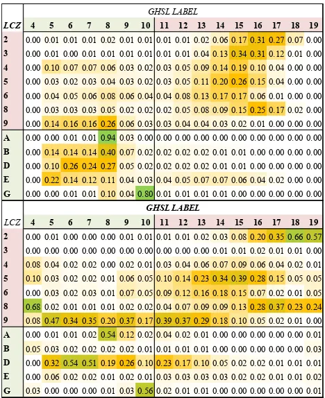
The results are presented in Table 4. While no clear relationship was found to exist between classes, there was generally good agreement between natural and urban types. An exception is LCZ 9 (sparsely built), which tended to be classified as various natural classes in LABEL This might be due to the image resolution which influences discrimination between the built and not built-up pixels (further classified as natural areas) of sparsely built landscapes. Good matches (> 50 % agreement) include LCZ A (dense trees) and LABEL 8 (forest) and LCZ G (water) and LABEL 10 (surface water) (both ways). Most of the LABEL 6 (rain cropland) and 7 (irrigated cropland) correspond with LCZ D (low plants). Both urban LABEL classes 18 and 19 (strong built-up, highrise and very highrise) correspond well with LCZ 2 (compact midrise). Surprisingly, the LABEL classes 4 (shrubs and grassland) show good agreement with LCZ 8 (large lowrise); however, the small sample size should be taken into account here. Generally, the dense urban label types (16-19) correspond with LCZs 2 (compact midrise) and 8 (large lowrise), which indicates that the LABEL scheme has more differentiation within the compact types. However, there is no agreement between LCZ 8 and LABEL 12. The light and medium built LABEL types (13-15, and 16 to a lesser degree) corresponded quite well with LCZ 5
and 9 rather than 6. This indicates an overestimation of LCZ 9 (sparsely built) in the LCZ classification. LCZ 4 was corresponding with different LABEL classes (15, 14, 16, 5, 13 in descending co-occurrence).
4 5 6 7 8 9 10 11 12 13 14 15 16 17 18 19
2 0.00 0.01 0.01 0.01 0.02 0.01 0.01 0.01 0.01 0.02 0.06 0.17 0.31 0.27 0.07 0.00
3 0.00 0.01 0.00 0.01 0.01 0.01 0.01 0.01 0.01 0.04 0.13 0.34 0.31 0.12 0.01 0.00
4 0.00 0.10 0.07 0.07 0.06 0.03 0.02 0.03 0.05 0.09 0.14 0.19 0.10 0.04 0.00 0.00
5 0.00 0.03 0.02 0.03 0.04 0.03 0.02 0.03 0.05 0.11 0.20 0.26 0.15 0.04 0.00 0.00
6 0.00 0.04 0.05 0.06 0.08 0.06 0.04 0.04 0.08 0.13 0.17 0.17 0.06 0.01 0.00 0.00
8 0.00 0.03 0.03 0.03 0.05 0.02 0.02 0.02 0.05 0.08 0.09 0.15 0.25 0.17 0.02 0.00
9 0.00 0.14 0.16 0.16 0.26 0.06 0.03 0.03 0.04 0.04 0.03 0.02 0.01 0.00 0.00 0.00
A 0.00 0.00 0.01 0.01 0.94 0.03 0.00 0.00 0.00 0.00 0.00 0.00 0.00 0.00 0.00 0.00
B 0.00 0.14 0.14 0.14 0.40 0.07 0.02 0.02 0.02 0.02 0.01 0.01 0.00 0.00 0.00 0.00
D 0.00 0.10 0.26 0.24 0.27 0.05 0.02 0.02 0.02 0.02 0.01 0.01 0.00 0.00 0.00 0.00
E 0.00 0.22 0.14 0.12 0.11 0.04 0.03 0.04 0.05 0.07 0.07 0.06 0.04 0.02 0.00 0.00
G 0.00 0.00 0.01 0.01 0.10 0.04 0.80 0.01 0.01 0.01 0.01 0.00 0.00 0.00 0.00 0.00
4 5 6 7 8 9 10 11 12 13 14 15 16 17 18 19
2 0.00 0.01 0.00 0.00 0.00 0.01 0.01 0.01 0.01 0.02 0.03 0.08 0.20 0.35 0.66 0.57
3 0.00 0.00 0.00 0.00 0.00 0.00 0.00 0.00 0.00 0.00 0.01 0.01 0.02 0.01 0.01 0.00
4 0.08 0.04 0.02 0.02 0.00 0.02 0.01 0.03 0.04 0.06 0.07 0.09 0.06 0.04 0.02 0.01
5 0.10 0.03 0.02 0.02 0.01 0.06 0.05 0.10 0.14 0.23 0.34 0.39 0.28 0.15 0.05 0.05
6 0.00 0.03 0.02 0.03 0.01 0.07 0.05 0.09 0.12 0.16 0.18 0.15 0.07 0.02 0.01 0.05
8 0.68 0.02 0.01 0.01 0.01 0.02 0.02 0.04 0.07 0.09 0.09 0.13 0.28 0.37 0.23 0.24
9 0.08 0.47 0.34 0.35 0.20 0.37 0.17 0.39 0.37 0.29 0.18 0.10 0.05 0.02 0.01 0.00
A 0.00 0.01 0.01 0.02 0.54 0.12 0.02 0.04 0.02 0.01 0.00 0.00 0.00 0.00 0.00 0.01
B 0.05 0.03 0.02 0.02 0.02 0.02 0.01 0.01 0.01 0.01 0.00 0.00 0.00 0.00 0.00 0.03
D 0.00 0.32 0.54 0.51 0.19 0.26 0.10 0.23 0.17 0.10 0.05 0.02 0.02 0.01 0.01 0.01
E 0.00 0.06 0.02 0.02 0.01 0.02 0.01 0.03 0.03 0.03 0.03 0.02 0.02 0.01 0.01 0.02
G 0.03 0.00 0.00 0.00 0.01 0.03 0.56 0.02 0.01 0.01 0.00 0.00 0.00 0.00 0.00 0.01 GHSL LABEL
GHSL LABEL LCZ
LCZ
Table 4. Contingency table between LABEL (columns) and LCZ (rows) for Milan (derived at higher resolution). Upper: weighted by LCZ occurrence; lower: weighted by LABEL occurrence. Red and green symbolize built and natural classes respectively. The International Archives of the Photogrammetry, Remote Sensing and Spatial Information Sciences, Volume XLI-B8, 2016
Figure 2. Classifications from LCZ (column 1) and LABEL (columns 2) for Beijing (BEI), Chicago (CHI), Honk Kong (HK), Khartoum (KHA), Lisboa (LIS), Madrid (MAD), Milano (MIL) and Sao Paulo (SAO). Columns 3 and 4 represent subsets of the domain. Colours are the codes as presented in Table 3. The International Archives of the Photogrammetry, Remote Sensing and Spatial Information Sciences, Volume XLI-B8, 2016
3.2 Built fractions
To account for the differences in resolution and typology, a comparison in a coarse grid resolution (1 km) was conducted next. Since the ordinal data cannot be downscaled in a straightforward manner, different sets of classes were generated for both typologies and the fraction of pixels falling into one of these classes was subsequently assessed. Table 5 shows the chosen sets as well as the correlation coefficients (R) and the mean absolute distances (MAD) between different sets (N.B. high R and low MAD indicates good spatial agreement).
R
LCZ set all built strong built light-medium commercial
set IDs 11-19 16-19 13-15 12
all built 1-10 0.77 0.52 0.73 0.54
no sparse 1-8, 10 0.93 0.76 0.85 0.43
compact & open 1-6 0.88 0.67 0.85 0.39
compact 1-3 0.58 0.79 0.33 -0.03
open 4-6 0.81 0.46 0.88 0.50
commercial 8 0.50 0.51 0.37 0.25
MAD (%) IDs 11-19 16-19 13-15 12
all built 1-10 24.3 42.2 35.1 46.1
no sparse 1-8, 10 7.2 17.0 11.5 21.4
compact & open 1-6 9.8 13.4 8.2 16.8
compact 1-3 23.3 4.4 12.7 4.4
open 4-6 12.2 12.5 6.1 13.8
commercial 8 22.1 5.3 11.7 5.1
GHSL LABEL
Table 5. Accordance between aggregated built fractions on a 1000 m grid using different sets of LABEL (columns) and LCZ (rows) classes. Correlation coefficient R, mean absolute distance (MAD) in %.
First, it can be seen that the agreement between all built classes from GHSL with the LCZ is much better if the sparse class is neglected (R= 0.93 versus R = 0.77 and MAD 7.2 versus MAD = 24.3), which underlines the previous finding that LCZ 9 is problematic for built-up characterization. The compact LCZ types correspond well with the strongly built GHSL types (R= 0.79, MAD = 4.4), and the open LCZ types correspond well with light and medium built types of the GHSL scheme (R = 0.88, MAD=6.1). This means that while the detailed classes differ significantly, the aggregated broader categories show substantial agreement, at least at a coarser resolution. Also here, we can observe higher agreement between LCZ 8 (large low buildings associated with commercial, light industry, and transportation use) and LABEL strong built (16-19) than LABEL built-up with highly reflecting roof (12).
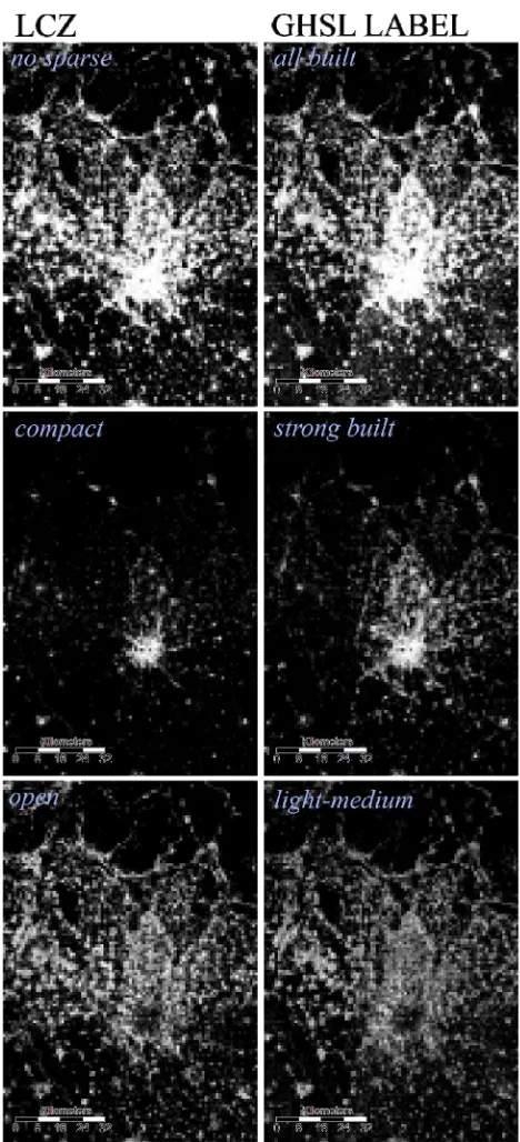
Figure 3 shows a spatial comparison between selected sets. Again is can be seen that LABEL (all built) and LCZ (no sparse) agree very well. Also the decomposition into compact/open (LCZ) and light-medium and strong built (LABEL) shows great similarity, even if the strong built class includes some additional structures out of the town center compared to the compact LCZ types. Figure 4 a) shows a scatterplot between the fractions of the sets LABEL (all built) and LCZ (no sparse), which also underlines the good general agreement in built-up areas. Figure 4 b) shows the fraction of different sets as a function of distance to town centre (in 5 km steps). The dashed lines represent LABEL sets while the solid lines are LCZ sets. Red represents the full built-up, black, the compact/strong built types and green the open/light-medium
types. The analysis confirms the good agreement of the full built up, with slightly higher fractions for LABEL (possibly due to the exclusion of LCZ 9). For the compact types, LABEL shows higher fractions, especially for the range from 10 to 35 km. This is consistent with the higher occurrence outside the town centre in Figure 3 and means that the class sets do not match perfectly. Otherwise, the agreement between the open types is very good for all distances. The artefacts beyond 70 result from the limited domain of the LCZ classification and the anisotropic structure of the city.
Figure 3. Accordance between different subsets on 1000 m grid. The International Archives of the Photogrammetry, Remote Sensing and Spatial Information Sciences, Volume XLI-B8, 2016
Figure 4. Left: Scatterplot between fraction of LABEL set all built and LCZ set built (without sparse). Right: mean radial fraction by distance from city centre for LABEL sets all built, strong built, light-medium and LCZ sets no sparse, compact, and open.
3.3 Detailed comparison
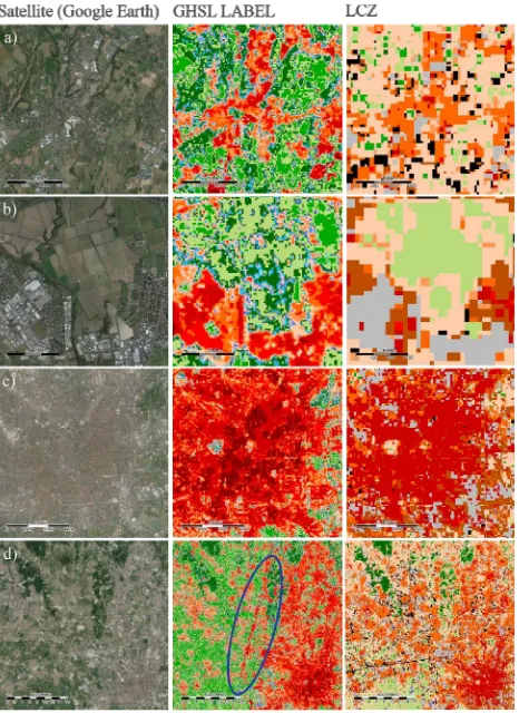
Finally, both classifications were investigated in more detail to assess some of the previous assumptions. Selected subsets are shown in Figure 5. Row a) illustrates the LCZ 9 problem, where the differentiation between agricultural areas (LCZ D) and lightly built areas is quite weak. This can also be seen in row b). Moreover, it can be seen that the large lowrise class (LCZ 8) is not mapped into the highly reflecting roof class in LABEL. Last, it can be seen that the LABEL classification is often noisy, with occurrence of different natural and built types, and mixed pixels tend to be classified into class 9 (Occasionally water / land-water interface), even if no water is present (probably due to shadows detected as water). Row c) shows the city centre. While the LCZ classification once again has a better discrimination of warehouse/commercial areas, the LABEL shows more differentiation within the densely built types due to the higher number of height classes. However, it still needs to be evaluated if these features can be found on the ground. Row d) eventually illustrates that LABEL sometimes shows artefacts like the linear structure highlighted by the blue ellipse. In this case, the error has been caused by a fog, which determined the classifier behaviour during in built-up detection.
4. CONCLUSIONS AND OUTLOOK
The next generation of global urban mapping products should focus on internal form and function of cities and not only built-up. LCZ and GHSL LABEL represent two approaches for generating better discretization of urban landscapes, both in experimental phase. LCZs are a generic typology of urban structures, which can be mapped using RS data and a supervised classifier. They have good empirical evidence in urban climatology but potentially a much wider scope in domains such as planning or emergency response. The GHSL LABEL is a global product derived by a methodology, developed for big remote sensing data scenarios. The built-up classes are derived by physical characteristics of settlement (i.e., built-up spatial density, height, roof reflectance, and vegetation presence). Both LCZ and LABEL have specific advantages and disadvantages. The typology of the LCZs provides information on a large number of climatic and physical properties, but the classification procedure needs city specific training data provided by experts. The GHSL processing workflow is fully automatic (i.e., no human intervention during all processing steps: input data selection, testing, training and classification), however, it highly depends on input data resolution and quality of training data (prone to errors).
Figure 5. Selected areas in Milan, colours as in Table 3.
Additionally, the LABEL classification schema is driven by physical rather functional properties of settlement.
The comparison between both datasets revealed a good agreement at city level and at coarse scale, while the agreement at pixel scale was – as expected – limited due to the mismatch in grid scale and typology. Generally, LABEL preserves more detail due to the higher resolution while for the LCZs, the internal structure seems somewhat clearer. At 1 km scale, the built-up areas showed very good agreement in terms of R and MAD, spatial pattern, and radial distribution as a function of distance from town. The same applies to aggregated class sets that represent open and compact (light/medium and strong built) classes, which could be matched quite well from both typologies. This finding is very relevant, since some studies indicate that a decomposition of urban area into just three classes might be sufficient for some modelling applications (Lee et al., 2011; Loridan et al., 2010). On the other hand, the commercial classes (LCZ 8: open lowrise, LABEL 12: highly reflecting roof) did not match. For the test case of Milan area, some specific problems were found for both datasets. For the LCZs, class 9 (sparsely built) was attributed to both built and natural landscapes. Thus, the training data needs immediate refinement here, while in the long run, a modification of the typology should be considered. Warehouse areas were not reflective enough to be classified as LABEL 12 and thus LCZs currently seem to be more capable to map this functional type. Furthermore, it revealed some artefacts and noise, with the frequent occurrence of class 9 (land-water interface) probably due to shadows classified as water.
We consider the first results of the comparison as preliminary but very promising, considering that the comparison is performed between products generated by semi-automatic and semi-automatic classifications. Also, the study has The International Archives of the Photogrammetry, Remote Sensing and Spatial Information Sciences, Volume XLI-B8, 2016
been performed on a subset of GHSL LABEL data and the quantitative analysis only on one test case. Thus, the study should be supplemented with different cities and revised, when the final LABEL product and improved LCZ versions are available. Further, a more detailed comparison, with additional spatial metrics and supplementary data (such as soil sealing, building height, LIDAR, OpenStreetMap) is envisaged. In addition, ways to combine both methodologies will be studied in the future. This includes the possibility to incorporate the LABEL 3D roughness into the LCZ classification, as well as refinement of the thresholds in LABEL to achieve higher consistency with the LCZ classes and thus better knowledge of the physical properties.
ACKNOWLEDGEMENTS
We thank all contributors to the WUDAPT database as well as the data providers (i.e. NASA, USGS and ESA).
REFERENCES
Alexander, P.J., Mills, G., Fealy, R., 2015. Using LCZ data to run an urban energy balance model. Urban Clim. 13, 14–37. doi:10.1016/j.uclim.2015.05.001
Bechtel, B., Alexander, P.J., Böhner, J., Ching, J., Conrad, O., Feddema, J., Mills, G., See, L., Stewart, I., 2015. Mapping Local Climate Zones for a Worldwide Database of the Form and Function of Cities. ISPRS Int. J. Geo-Inf. 4, 199–219. doi:10.3390/ijgi4010199
Bechtel, B., Daneke, C., 2012. Classification of Local Climate Zones Based on Multiple Earth Observation Data. IEEE J. Sel. Top. Appl. Earth Obs. Remote Sens. 5, 1191–1202. doi:10.1109/JSTARS.2012.2189873
Bechtel, B., See, L., Mills, G., Foley, M., 2016. Classification of Local Climate Zones Using SAR and Multispectral Data in an Arid Environment. IEEE J. Sel. Top. Appl. Earth Obs. Remote Sens. PP, 1–9. doi:10.1109/JSTARS.2016.2531420
Bontemps, S., Defourny, P., Bogaert, E.V., Arino, O., Kalogirou, V., Perez, J.R., 2011. GLOBCOVER 2009-Products description and validation report.
Brousse, O., Martilli, A., Foley, M., Mills, G., Bechtel, B., 2016. WUDAPT, an efficient land use producing data tool for mesoscale models? Integration of urban LCZ in WRF over Madrid. Urban Clim. accepted.
Ching, J.K.S., 2013. A perspective on urban canopy layer modeling for weather, climate and air quality applications. Urban Clim. 3, 13–39. doi:10.1016/j.uclim.2013.02.001
Conrad, O., Bechtel, B., Bock, M., Dietrich, H., Fischer, E., Gerlitz, L., Wehberg, J., Wichmann, V., Böhner, J., 2015. System for Automated Geoscientific Analyses (SAGA) v. 2.1.4. Geosci Model Dev 8, 1991–2007. doi:10.5194/gmd-8-1991-2015
Esch, T., Marconcini, M., Felbier, A., Roth, A., Heldens, W., Huber, M., Schwinger, M., Taubenbock, H., Muller, A., Dech, S., 2013. Urban footprint processor—Fully automated processing chain generating settlement masks from global data of the TanDEM-X mission. IEEE Geosci. Remote Sens. Lett. 10, 1617–1621. doi:10.1109/LGRS.2013.2272953
Gamba, P., Lisini, G., Liu, P., Du, P., Lin, H., 2012. Urban climate zone detection and discrimination using object-based analysis of VHR scenes. Proc. 4th GEOBIA 7–9.
Heiden, U., Heldens, W., Roessner, S., Segl, K., Esch, T., Mueller, A., 2012. Urban structure type characterization using hyperspectral remote sensing and height information. Landsc.
Urban Plan. 105, 361–375. doi:10.1016/j.landurbplan.2012.01.001
Jackson, T.L., Feddema, J.J., Oleson, K.W., Bonan, G.B., Bauer, J.T., 2010. Parameterization of Urban Characteristics for Global Climate Modeling. Ann. Assoc. Am. Geogr. 100, 848– 865. doi:10.1080/00045608.2010.497328
Lee, S.-H., Kim, S.-W., Angevine, W.M., Bianco, L., McKeen, S.A., Senff, C.J., Trainer, M., Tucker, S.C., Zamora, R.J., 2011. Evaluation of urban surface parameterizations in the WRF model using measurements during the Texas Air Quality Study 2006 field campaign. Atmospheric Chem. Phys. 11, 2127–2143.
Lelovics, E., Unger, J., Gál, T., Gál, C.V., 2014. Design of an urban monitoring network based on Local Climate Zone mapping and temperature pattern modelling. Clim. Res. 60, 51– 62. doi:10.3354/cr01220
Loridan, T., Grimmond, C.S.B., Grossman-Clarke, S., Chen, F., Tewari, M., Manning, K., Martilli, A., Kusaka, H., Best, M., 2010. Trade-offs and responsiveness of the single-layer urban canopy parametrization in WRF: An offline evaluation using the MOSCEM optimization algorithm and field observations. Q. J. R. Meteorol. Soc. 136, 997–1019.
Pachauri, R.K., Allen, M.R., Barros, V.R., Broome, J., Cramer, W., Christ, R., Church, J.A., Clarke, L., Dahe, Q., Dasgupta, P., others, 2014. Climate Change 2014: Synthesis Report. Contribution of Working Groups I, II and III to the Fifth Assessment Report of the Intergovernmental Panel on Climate Change.
Pesaresi, M., Ferri, S., Ehrlich, D., Florczyk, A.J., Freire, S., Halkia, M., Julena, A., Kemper, T., Soille, P., Syrris, V., 2016a. Operating procedure for the production of the global human settlement layer from Landsat data of the epochs 1975, 1990, 2000, and 2014, JRC Technical Report.
Pesaresi, M., Huadong, G., Blaes, X., Ehrlich, D., Ferri, S., Gueguen, L., Halkia, M., Kauffmann, M., Kemper, T., Lu, L., Marin-Herrera, M.A., Ouzounis, G.K., Scavazzon, M., Soille, P., Syrris, V., Zanchetta, L., 2013. A Global Human Settlement Layer From Optical HR/VHR RS Data: Concept and First Results. IEEE J. Sel. Top. Appl. Earth Obs. Remote Sens. 6, 2102–2131. doi:10.1109/JSTARS.2013.2271445
Pesaresi, M., Syrris, V., Julena, A., 2016b. ANALYZING BIG REMOTE SENSING DATA VIA SYMBOLIC MACHINE LEARNING, in: Soille, P., Marchetti, P.G. (Eds.), Proceedings of the 2016 Conference on Big Data from Space (BiDS’16), 15–17 March 2016, Santa Cruz de Tenerife, Spain. pp. 156– 159.
Schneider, A., Friedl, M.A., Potere, D., 2009. A new map of global urban extent from MODIS satellite data. Environ. Res. Lett. 4, 44003. doi:10.1088/1748-9326/4/4/044003
Stewart, I.D., 2011. A systematic review and scientific critique of methodology in modern urban heat island literature. Int. J. Climatol. 31, 200–217. doi:10.1002/joc.2141
Stewart, I.D., Oke, T.R., 2012. Local Climate Zones for Urban Temperature Studies. Bull. Am. Meteorol. Soc. 93, 1879–1900. doi:10.1175/BAMS-D-11-00019.1
Voltersen, M., Berger, C., Hese, S., Schmullius, C., 2015. Expanding an urban structure type mapping approach from a subarea to the entire city of Berlin, in: Urban Remote Sensing Event (JURSE), 2015 Joint. IEEE, pp. 1–4.