OPERATIONAL SEMI-PHYSICAL SPECTRAL-SPATIAL WHEAT YIELD MODEL
DEVELOPMENT
R Tripathy a, *, K.N. Chaudhary a, R.Nigam a, K.R. Manjunath a, P. Chauhan a, S.S. Ray b, and J.S. Parihar a a EPSA, Space Applications Centre, Ahmedabad, India - (rose_t, kishan, rahulnigam, krmanjunath, prakash,
jsparihar)@sac.isro.gov.in b
MNCFC, New Delhi, India ([email protected])
KEY WORDS: Monteith efficiency model, Remote sensing, LSWI, MODIS, K1-VHRR, RS2-AWiFS, regional wheat yield
ABSTRACT:
Spectral yield models based on Vegetation Index (VI) and the mechanistic crop simulation models are being widely used for crop yield prediction. However, past experience has shown that the empirical nature of the VI based models and the intensive data requirement of the complex mechanistic models has limited their use for regional and spatial crop yield prediction especially for operational use. The present study was aimed at development of an intermediate method based on the use of remote sensing and the physiological concepts such as the photo-synthetically active solar radiation (PAR) and the fraction of PAR absorbed by the crop (fAPAR) in Monteith’s radiation use efficiency based equation (Monteith, 1977) for operational wheat yield forecasting by the Department of Agriculture (DoA). Net Primary Product (NPP) has been computed using the Monteith model and stress has been applied to convert the potential NPP to actual NPP. Wheat grain yield has been computed using the actual NPP and Harvest index. Kalpana-VHRR insolation has been used for deriving the PAR. Maximum radiation use efficiency has been collected from literature and wheat crop mask was derived at MNCFC, New Delhi using RS2-AWiFS data. Water stress has been derived from the Land Surface Water Index (LSWI) which has been derived periodically from the MODIS surface reflectance data (NIR and SWIR1). Temperature stress has been derived from the interpolated daily mean temperature. Results indicated that this model underestimated the yield by 3.45 % as compared to the reported yield at state level and hence can be used to predict wheat yield at state level. This study will be able to provide the spatial wheat yield map, as well as the district-wise and state level aggregated wheat yield forecast. It is possible to operationalize this remote sensing based modified Monteith’s efficiency model for future yield forecasting with around 0.15 t ha-1 RMSE at state level.
1. INTRODUCTION
Since the advent of Earth-observing satellites several decades ago, researchers have made efforts to derive useful information about agricultural fields from satellite data. Agricultural production can be affected by many factors, such as technological, biophysical or climatological factors. Many of these drivers can be assimilated /modeled or estimated using remote sensing approaches. Estimation of actual crop yield through remote sensing offers an alternative to the more resource-consuming field measurements and surveys typically used to estimate crop yields at regional to national scales. There are many methods of crop yield estimation prior to harvest using remote sensing. Models for yield estimation have been developed from empirical to physiological growth simulation models. Vegetation index (VI) based empirical models are location-specific and cannot be extrapolated over larger areas with adequate accuracy (Moulin et al., 1998). Moreover, the coefficients call for updation after few years. They could explain only 50 to 60% yield variability. Hence these models were replaced with mechanistic and dynamic crop growth simulation model (CSM) that can physiologically and quantitatively describe the response of plants to their environment. Though these models describe the primary physiological mechanisms of crop growth and development in a computational loop, the difficulties of adopting CSM has usually been associated with the intensive data requirement for models’ parameterization. The need for calibration can be quite data extensive and hence not applicable for large area yield estimation. The use of these models in large areas has been limited also because most plant growth models were developed
at the field scales and hence, inadequate to run at regional/national scale. The intrinsic differences between some of the variables measured on the ground and the variables derived from satellite have limited the assimilations of those variables in these mechanistic crop simulation models.For example, surface temperature derived from a satellite radiometer at noon often differs considerably from daily maximum air temperature measured at 2 m on the ground (de Wit et al., 2004). This makes integration of such variables in crop simulation models difficult because many biophysical relationships within these models (assimilation, respiration, etc.) have been calibrated on air temperature rather than radiometric surface temperature.
Looking at the pros and cons of the empirical VI based models as well as the complex crop simulation models, it is wise to think of an ensemble regional crop yield forecast method taking the advantage of all these approaches to arrive at confident and conclusive end results. Hence an intermediate method has been planned for regional wheat yield estimation based on the use of remote sensing and the physiological concepts such as the photosynthetically active solar radiation (PAR) and the fraction of PAR absorbed by the crop (fAPAR) in Monteith’s efficiency equation (Monteith, 1977). PAR and fAPAR can help to assess the real-time information of the crop growing conditions at any stage during the crop growing season. The parameters of model were not empirical estimates, but were derived using physiological concepts. The Vls and greenness are linearly related to PAR absorption rate of crop canopies and hence, crop absorbed PAR can be estimated from remotely sensed VI or greenness and PAR observed at ground stations. This has been utilized for many crops to remotely estimate yields with
satisfactory results (Asrar et al., 1985: Wiegand et al., 1989: Wiegandet al., 1990).
This method, however, gives a potential crop yield rather than an actual yield. The constant radiation conversion efficiency and constant harvest index are assumed. Radiation conversion efficiency is affected by nitrogen deficiency (Sinclair & Horie, 1989) and water stress, while harvest index is influenced by water or temperature stress during reproductive and grain-filling stages. The nitrogen deficiency is accounted by fAPAR (NDVI), hence the major stress left are water and temperature stress. The present study was carried out with the objective of developing a semi-physical spectral yield model for operational forecast of wheat yield at regional scale using remotely sensed biophysical parameters.
2. MATERIALS AND METHOD 2.1 Study area
1.1 The six major wheat growing states (Punjab, Haryana, Rajasthan, MP, UP and Bihar) were taken as the study area for the investigation. These six states constitute around 85% of the total wheat growing area and contribute about 90% of the total wheat production of the country. Punjab, Haryana and Western-UP constitute the major irrigated wheat area while Rajasthan, MP and Bihar states constitutes most of the rain-fed area under wheat.
2.2 Methodology
The methodology is based on the concept that the biomass produced by a crop is a function of the amount of photosynthetically active radiation (PAR) absorbed, which in turn depends on incoming radiation and the crop's PAR interception capacity. The first steps that helped researchers to link RS and PAR was the equation developed by Monteith in 1977 to quantify the fAPAR (Monteith, 1977). fAPAR is defined as the fraction of absorbed PAR (APAR) to incident PAR (0 < fAPAR < 1): fAPAR = APAR/PAR and is quantified from RS because it has been found a good predictive ability by NDVI (Baretet al.,1989). The mechanism by which the incident PAR is transformed into dry matter can be written as:
(1)
Where ΔDM= dry matter accumulation in plant over a period of time or NPP (g•m−2•d−1)
PAR = incident photosynthetically active radiation (MJ•m−2•d−1)
fAPAR= fraction of incident PAR which is intercepted and absorbed by the canopy (dimensionless)
ε = Light-use efficiency of absorbed photosynthetically active radiation (g•MJ−1)
The light-use efficiency (ε) is relatively constant for crops like wheat (with a value of about 3.0 g•MJ−1) when calculated over
the entire growth cycle and in the absence of growth stresses (Stockle and Nelson, 1996). However, the light-use efficiency is not constant when calculated over small periods of the growth cycle. The short-term variability of the light-use efficiency is a result of temperature, nutrient and water conditions that eventually can lead to plant stress. The seasonal integration of radiometric measurements theoretically improves the capability of estimating biomass compared to one-time measurements (Baret et al., 1989; Rembold et al. 2013). In the present study
PAR, fAPAR and the stress factors was acquired/computed over the whole wheat season (mid October to end April) at a temporal resolution of 8 days and then integrated. Thus the Monteith’s efficiency equation has been extended to include, impact of water stress (Wstress) and temperature stress (Tstress) on photosynthesis and hence the modified equation becomes
(2)
It was reported that the SWIR band (1.6 µm) was sensitive to plant water content (Tucker, 1980, Xiao et al., 2004). In the present study the water stress has been computed from an index calculated as the normalized difference between the NIR (0.78– 0.89 Am) and SWIR (1.58–1.75 µm) spectral bands, which is called the Land Surface Water Index (LSWI) (Xiao et al., 2002c, 2004). The water stress can be computed as:
(3)
LSWI max has been taken as the spatial maximum of all states on a particular day. LSWI for particular pixel can be computed as:
(4) Tstressis estimated at each time step, using the equation (Raich et al., 1991):
(5) Where Tmin=minimum temperature for photosynthesis (°C)
Tmax= maximum temperature for photosynthesis (°C) Topt= optimal temperature for photosynthesis (°C) T= the daily mean temperature (°C)
For wheat, Tmin: 5°C; Tmax=35°C and Topt=25°C. If air temperature falls below Tmin, Tscalar is set to be zero.
The economic grain yield is the product of harvest index (HI) and net primary productivity (NPP). That is:
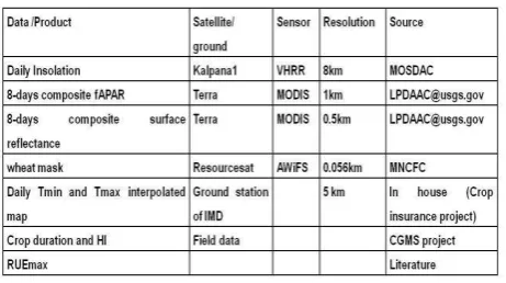
(6) The grain yield for a state is computed as aweighted average of pixel grain yield of wheat pixels in a region.The methodology is based on the above mentioned approach which is graphically presented in Figure 1. Periodical NPP (8 days) was integrated from planting date to harvest date which varies with state. The crop duration and harvest index were taken from the data collected in previous study on Crop Growth Monitoring System (Chaudhari et al., 2010; Tripathy et al., 2013). Wheat mask was applied to compute the total NPP or biomass and grain yield of wheat pixel. The pixel yield was averaged to district level and average state yield was computed. Table 1 shows the source and other information for the data used in the study.
Figure 1. Methodology for wheat yield estimation using RS based modified Monteith model (ε: light-use efficiency of crop, fAPAR: fraction of incident photosynthetically active radiation (PAR) which is intercepted and absorbed by the canopy, Tav: average daily temperature, : Reflectance in the respective wave
lengths, APAR: Total PAR absorbed by the canopy LSWI: Land Surface Water Index, HI: harvest index) Table 1: The list of data used with their sources
2.3 Data processing and computation of parameters 2.3.1 Image acquisition and processing of KVHRR- insolation product:Daily Insolation data product has been downloaded from MOSDAC (www.mosdac.gov.in) over the crop season i.e., from 15 Oct 2013 to 21 March 2014; and past data from last three years for a period from 22 March to 30 April. The processing of daily insolation involved the conversion of daily insolation to 8 day product (sum) and resampling to 1 km resolution.50 % of the total insolation was assumed as photo-synthetically active radiation or PAR. 2.3.2 Image acquisition and processing of MODIS data product: MODIS surface reflectance products (8 day composites) with 0.5km spatial resolution; fAPAR product (8day composites) with 1km resolution has been downloaded from (https://lpdaac.usgs.gov). MODIS products are in HDF format distributed using the sinusoidal projection.
MOD09A1 or MODIS Surface Reflectance 8-Day L3 Global 500m file is a composite using eight consecutive daily 500 m images. The best observation during each eight day period, for every cell in the image, is retained. This helps reduce or eliminate clouds from a scene. The file contains seven spectral bands of data as the daily file. It also has an additional 6 bands of information concerning quality control, solar zenith, view zenith, relative azimuth, surface reflectance 500 m state flags, and surface reflectance day of year.
MODIS bands for reflectance measurement
MODIS has 7 bands in the visible and infrared region. The band width of these bands are:- Band 1: 0.620-0.670 µm; Band 2: 0.841-0.876 µm; Band 3: 0.459-0.479 µm;Band 4: 0.545-0.565
µm; Band 5: 1.230-1.250 µm; Band 6: 1.628-1.652 µm and Band7: 2.105-2.155 µm.
The MOD13A1 data product contains the MODIS/TERRA Vegetation Indices 8-day L3 Global 1km data from Terra for an 8-day composite at 1km resolution in the sinusoidal projection. MOD09A1 and MOD13A1 data products were acquired over the wheat season (15 Oct-15 March of the current season and 16 March to 30 April of the last three years), and processed. The processing of MODIS data included the mosaicking of tiles for India, resizing to India boundary, conversion to geographical projection from the sinusoidal projection and resampling of surface reflectance to 1km. The past data were used for the period from the date of data processing for forecasting till the end of the crop season. Average of three consecutive year’s data (2011, 2012 and 2013) was taken for computing the normal fAPAR. LSWI was computed using the band 2 (NIR-0.841-0.876µm) and 6 (SWIR1: 1.628-1.652 µm) using eq. 4. From LSWI water stress was computed at 1km spatial resolution using eq 3.
2.3.3 Computation of temperature stress: Daily average temperature has been computed from the daily maximum and minimum temperature of IMD weather data interpolated to 5 km grid. The daily temperature stress in a scale of 0-1 has been computed using eq5. The average temperature stress over an 8 days period was computed and all images were converted to 1x1 km resolution.
2.3.4 Computation of Net Primary Product and grain yield: NPP has been computed for a period of sowing to harvest at an interval of 8 days for each state with a spatial resolution of 1km using the periodical PAR, fAPAR, Wscalar, Tscalar and maximum radiation use efficiency in eq2. Total NPP has been computed for each state using the crop duration from CGMS project and sowing date from normal crop calendar for the respective state. From the total NPP grain yield per pixel has been computed using eq 6. Wheat mask was applied to compute the average grain yield at district and state level. For averaging only wheat pixels as derived from AWiFS were considered. 2.4 Evaluation of Results
The methodology has been evaluated by comparing the estimated grain yield with the average of last five years reported yield taken from Department of Agriculture and Cooperation (DAC). The grain yield has been compared at state and district level. Absolute difference and the RMSE statistic have been used for comparison.
3. RESULTS AND DISCUSSION
3.1 Water and temperature stress
The water stress was applied upto flowering stage of the crop growth. Among the six wheat states, maximum water stress was observed in MP in the month of Feb. In Punjab water stress in scale of 0-1 varied from 0.7 (maximum stress) to 1 (no stress). Image of LSWI and the corresponding water stressmap for an 8 day period (from 25 Jan to 1 Feb) has been depicted in Figure 2.The same trend was observed for other dates also.
Figure 2: LSWI and Water stress map of India (1: no stress; 0: maximum stress)
Average temperature stress in a scale of 0-1over a period of 8 days as derived from the average interpolated temperature has been depicted in Figure 3. For this period the temperature stress was highest for Punjab and Haryana because of low temperature for wheat growth. The trend changed with the advancement of summer and highest stress was observed in MP, Bihar towards end March.
Temperature stress map of India
Period: 25Jan- 1 Feb 2014
Tx Tn
Tmean
Figure 3: Temperature stress map of India (1: no stress; 0: maximum stress)
3.2 NPP and grain yield
NPP has been computed state wise over the growing period at an interval of 8 days using the state-wise maximum radiation use efficiency of the major cultivar in the respective state. NPP of Punjab state for an 8 days period (25 Jan to 1 Feb) has been depicted below (Figure 4). Total NPP from planting to harvest has been computed after applying wheat mask. The NPP in different pixel in the depicted scene ranged from 25 to 77 g m-2. NPP for other states are computed in the same manner.
Figure 4: NPP (g m-2) of Punjab for an 8 days period (25 Jan-1 Feb)
Grain yield was computed from total NPP using the harvest index of the respective cultivar in each state. The state wise estimated grain yield ranged from 2.123 t ha -1 in MP to 4.623 t ha-1 in Punjab.Spatial variability within a state is depicted in Figure 5. In most of the pixel in Punjab and Haryana state the yield ranged from 3-6 t ha-1. In Bihar the yield ranged from1-3 t ha-1. In MP it ranged from 0.7 to 4 t ha-1 while in most of the pixels of UP and Rajasthan the yield ranged from 2-5 t ha-1 (Figure 5).
Punjab Haryana Bihar
Rajasthan Uttar Pradesh Madhya
Pradesh
Figure 5: Spatial wheat yield (t ha-1) of the six study states 3.3 Evaluation of the methodology
The state level comparison with the reported yield indicated anaverage underestimation of 3.45 %. In each state the estimation remained below the reported yield except for Punjab where it is slightly more than the reported yield. Except for MP the state level difference between estimated and reported was within 10 % and the resulted RMSE was estimated to be 0.15 t ha-1 (Table 2, Figure 6). The absolute difference between reported and simulated grain yield was found to be least in Punjab (0.13 %) and highest in MP (11.79 %). The RMSE between observed and estimated wheat yield in different states was found to be 0.15 t ha-1.
Table 2: Comparison of estimated yield with reported yield (GY_est: estimated yield (t ha-1); GY_rep: reported yield (t ha-1) Diff: percentage deviation from the reported yield
Dist GY_est_14
GY_rep_13-14
Diff (%)
Bihar 2.15 2.35 -8.75
Haryana 4.47 4.55 -1.79
MP 2.12 2.41 -11.76
Punjab 4.62 4.62 0.13
Rajasthan 3.09 3.18 -2.78
UP 3.03 3.08 -1.43
Average 3.25 3.36 -3.45
S
imulated
Gr
ain
Y
ie
ld
(t/ha)
Observed Grain Yield (t/ha) 0.00
1.00 2.00 3.00 4.00 5.00
0.00 1.00 2.00 3.00 4.00 5.00
1:1 line
10% line
R2=0.996 RMSE=0.15 t ha-1
Figure 6: Comparison of estimated yield with reported yield
District level yield was compared with the average district level reported yield of past five years (2007-11) as current season reported yield at district level is not available. Results indicated that, in Punjab and Haryana the absolute difference is within
Figure 7: Comparison of estimated wheat yield in the study states with the average of past five year’s historical yield at
district level
Possible reason for disparity in spatial yield may be attributed to the error in planting date. For this study, we applied same weight for the yield with different sowing dates in all districts of a state, e.g. in Punjab we had taken three sowing dates (50 % for 15 Nov, 25 % for 1 Dec and 25 % for 15 Dec) and the same weight has been used for Ludhiana as well as for Bathinda (cotton growing with maximum late planted wheat area). We hope with the use of spatial planting date from remote sensing we will be able to overcome the district level yield disparity.
4 CONCLUSION
The current approach has been tested on regional scale for six major wheat growing states of India as input to operational forecast of wheat yield at MNCFC, Department of Agriculture & Cooperation (DAC). The results from this study demonstrated that this model can be used to predict wheat yield at state level. This study will be able to provide the spatial wheat yield map, as well as the district-wise and state level aggregated wheat yield forecast. This spectral wheat yield model provides wheat yield with about 0.15 t ha-1 Agricultural output using Space Agro-meteorology and Land based observations)-R&D project at Space Application Centre, Ahmedabad funded by DAC, Ministry of Agriculture. We express our gratitude to the ministry for providing financial support to the project. We are grateful to Shri A. S. Kiran Kumar, Director, Space Applications Centre, for his encouragement and keen interest in this study. Authors are
grateful to Dr. P. K. Pal, DD,EPSA for extending his support for this study. We acknowledge MOSDAC for the daily insolation data and NASA (lpdaac.usgs.gov) for MODIS reflectance and FAPAR data.
REFERENCES
Asrar, G., Kanemasu, E.T., Jackson, R.D., Pinter Jr., P.J. 1985. Estimation of total above-ground phytomass production using remotely sensed data. Remote Sensing of Environment, 17: 211–220.
Baret, F., Guyot, G., Major, D.J. 1989.Crop biomass evaluation using radiometric measurements.Photogrammetria, 43: 241– 256.
Chaudhari K.N., Tripathy, R., Patel, N.K., 2010. Spatial wheat yield prediction using crop simulation model, GIS, remote sensing and ground observed data. Journal of Agrometeorology, 12(2):174-180.
de Wit, A.J.W., Boogaard, H.L. van Diepen, C.A. 2004. Using NOAA-AVHRR estimates of land surface temperature for regional agrometeorogical modelling, International Journal of Applied Earth Observation and Geoinformatics, 5: 187–204. Monteith, J.L. Climate and the efficiency of crop production in Britain. 1977. Phil. Trans. R. Soc. London., 281: 277–294. Moulin, S., Bondeau, A, Delécolle, R. 1998. Combining agricultural crop models and satellite observations: From field to regional scales. International. Journal of Remote Sensing, 19: 1021–1036.
Raich, J. W., Rastetter, E. B., Melillo, J. M., Kicklighter, D. W., Steudler, P. A., Peterson, B. J., Grace, A. L., Moore, B., Vorosmarty, C. J. 1991. Potential net primary productivity in South-America—application of a global-model. Ecological Applications, 1: 399–429.
Rembold , F., Atzberger, C., Savin, I., Rojas,O. 2013. Using Low Resolution Satellite Imagery for Yield Prediction and Yield Anomaly Detection. Remote Sensing , 5: 1704-1733; Manual(Version 2.0) Biological Systems Engineering Department,Washington State University, Pullman, WA, USA. Tripathy R., Chaudhari, K.N., Mukherjee, j., Ray, S.S., Patel, N.K., Panigrahy, S., Parihar, J.S., 2013. Forecasting wheat yield in Punjab state of India by combining crop simulation model WOFOST and remotely sensed inputs. Remote Sensing Letters, 4:1, 19-28.
Tucker, C. J. 1980. Remote-sensing of leaf water-content in the near infrared.Remote Sensing of Environment, 10: 23– 32. Wiegand, C., Shibayama, M., Yamagata, Y., Akiyama, T., 1989.Spectral observations for estimating the growth and yield of rice. Japanese Journal of Crop Science, 58: 673–683.
Wiegand, C.L., Gerbermann, A.H., Gallo, K.P., Blad, B.L., Dusek, D. 1990. Multisite analyses of spectral-biophysical data for corn. Remote Sensing of Environment, 33: 1-16.
Xiao, X., Boles, S., Liu, J. Y., Zhuang, D. F., Liu, M. L. 2002c. Characterization of forest types in Northeastern China, using multitemporal SPOT-4 VEGETATION sensor data. Remote Sensing of Environment, 82: 335– 348.
Xiao, X., Hollingerb, D., Abera, J., Goltzc, M., Davidsond, E. A., Zhanga,Q., Moore, B. 2004. Satellite-based modeling of gross primary production in an evergreen needle leaf forest. Remote Sensing of Environment, 89: 519–534.