www.elsevier.comrlocateratmos
A double moment warm rain scheme: description
and test within a kinematic framework
Gustavo G. Carrio
´
), Matilde Nicolini
Departamento de Ciencias de la Atmosfera, Centro de In´ Õestigaciones del Mar y la Atmosfera, Consejo´ Nacional de InÕestigaciones Cientıficas y Tecnologicas, Uni´ ´ Õersidad de Buenos Aires, Buenos Aires,
Argentina
Received 14 September 1998; received in revised form 4 February 1999; accepted 10 June 1999
Abstract
A two-moment warm rain parameterization that includes prognostic equations for mixing ratios and number concentrations is described. The number of activated condensation nuclei is also prognosed assuming a log–linear relationship between the total number of activated condensation nuclei and the supersaturation. Collective processes are evaluated using pre-calculated matrices of interaction based on numerical integrations of the corresponding stochastic collection equations. Mass transfer between cloud and raindrops due to autoconversion is evaluated using Berry’s parameterization, its attendant raindrop number concentration change is calculated considering the corresponding rates of change for the first and second moments of the raindrop volume distribution. A Doppler kinematic reconstruction of a summertime Hawaiian rainband occurred on
August 10, 1990 is used to evaluate the credibility of this scheme.q1999 Elsevier Science B.V.
All rights reserved.
Keywords: Warm rain; Autoconversion; Microphysical schemes
1. Introduction
Ž .
Many cloud modelers have used the so-called Kessler 1969 parameterization to evaluate the transformation between categories in which water substance is classified. Its benefits mainly lie in its inexpensiveness in term of computer resources as it takes as prognostic variables only the mixing ratios of the different species. On the other hand,
)Corresponding author
0169-8095r99r$ - see front matterq1999 Elsevier Science B.V. All rights reserved.
Ž .
the state of art of modeling of explicit spectral microphysics was developed during the eighties considering detailed spectral treatments of processes such as
collision–coales-Ž
cence, collisional breakup and nucleation Kogan, 1991; Feingold et al., 1991, among
.
others . Explicit treatments ensure an adequate description of the various processes, however they require an enormous computer capacity when they are considered within a multidimensional dynamic framework. There is a trend in recent years to include prognostic equations for an additional moment of the species distributions, namely
Ž .
number concentrations Ferrier, 1994; Walko et al., 1995; Meyers et al., 1997 . Multimoment schemes appear to be a compromise solution between the detail of the description and computational expedience. A mixed phase microphysical package that includes prognostic equations for mixing ratios and number concentrations of various water species is being developed by the authors, its warm rain scheme is here described and tested with observational data.
Ž .
During the Hawaiian Rainband Project HaRP several aspects of a series of shallow tropical rainbands offshore of the island of Hawaii have been studied. Dual-Doppler radar measurements from this project have been used to document the formation,
Ž .
evolution and kinematic structure of high reflectivity cores Szumowski et al., 1997 . A two-dimensional dual-Doppler kinematic reconstruction of a rainband, designed to test
Ž .
warm rain microphysical packages Szumowski et al., 1998a , is used here to evaluate the credibility of the above mentioned two moment warm rain scheme. This reconstruc-tion represents one of the best cases documenting kinematics and the time evolureconstruc-tion of high reflectivity cores in warm rain clouds. Within a kinematic framework, the absence of microphysical–dynamical interactions, such as loading effects, certainly introduces limitations, although, it allows isolating the response of different microphysical parame-terizations and schemes. Some aspects of the simulated microphysical structure are compared with those of a rainband occurred on July 23, 1985, documented and analyzed
Ž .
by Szumowski et al. 1998b using aircraft data. A general description of the scheme is given in Section 2. The comparison between simulated and observed characteristics and final comments are presented in Sections 3 and 4, respectively.
2. Scheme description
Cloud droplet and raindrop volume spectra are assumed to follow gamma
distribu-Ž .
tions of the type used by Berry and Reinhardt 1974 . The volume corresponding to a drop of 40mm in radius is taken as the boundary between both spectra as it corresponds to the nearly stationary position of a minimum when solving the stochastic collection equation.
n nq1
N
Ž .
Õ sNtŽ
nq1.
Ž
ÕrÕf.
r ÕfG nŽ
q1.
exp yŽ
nq1.
ÕrÕfŽ .
1Ž .
where N Õ is the number density of drops with volume Õ, N is the total numbert
Ž . Ž .
concentration,Õf is the mean volume,n is a width parameter n)y1 and G x is the
The relation between the volume about which most of the mass is concentrated
Žpredominant volume and the mean volume and the width parameter is given in Eq. 2 .. Ž .
Any moment of the gamma volume distribution can be evaluated in terms of the
Ž .
spectrum parameters with Eq. 3 .
y1
y1
y1
w x
1 0 2 1nq1 s Õ Õ y1s M rM M rM y1 2
Ž
.
f gŽ .
where Õ is the predominant volume and Mb denotes the bth moment of the volume
g
The mixing ratios of cloud droplets and raindrops Q and Qc r and the corresponding
Ž .
number concentrations N and N along with the concentration of activated nuclei, arec r
Ž .
taken as prognostic variables, however the width parameters nc andnr are assumed to remain constant during the simulation. The chosen values are consistent with observa-tions in Hawaiian clouds and they are 0 fornc andy0.8 for nr.
Ž . Ž .
The following Eqs. 4 – 8 represent the tendency equations for Q , Q , N , N andc r c r
Ž .
the number concentration of activated nuclei N .n
< < < where the subscript, NUC, CON, AUT, ACR, SFC, ADV, SED and EVA stand for nucleation, condensation, autoconversion, accretion, raindrop self-collection, advection, sedimentation and evaporation, respectively.
2.1. Collisional processes
2.1.1. AutoconÕersion
Ž .
Following Berry and Reinhardt 1974 , an average autoconversion rate can be
Ž .
evaluated relating a characteristic liquid water content change L2 and a corresponding
Ž .
time scale t2 . The resulting tendency equation for Q due to autoconversion is givenc
Ž . Ž
in Eq. 9 as a function of the cloud drop spectrum parameters cgs units are used
.
hereafter .
< <
where
rfc is the mean volume droplet radius and r is the air density.
Ž .
Under the constraint of a constant value for the raindrop width parameter nr , the corresponding rates of change for the first and second moments and the number
Ž 0.
concentration M are not independent. Therefore, the time rate of change for N due tor
autoconversion is here evaluated in terms of the corresponding rates of change of M1 and M2 and assuming that the newly created raindrops have a mean volume coincident
with the chosen boundary between both spectra.
Ž .
The raindrop mean volume Õ and the more physically meaningful predominant
fr
Ž . Ž Ž ..
volume Õ are linearly related for a givenn see Eq. 2 . If rate of change for N due
gr r r
Ž .
to autoconversion is evaluated relating Eq. 9 to the volume of a drop of 40mm, Õ
gr
and the radar reflectivity are then artificially decreased by the inclusion of these small drops.
The raindrop predominant volume after a time interval Dt can be related to <
dQrrd tAU T using the following equation:
2U 2 2 < U U
M sMr qDMAUTsr a
Ž
r frÕ.
Qrqr aŽ
AUT 40Õ.
dQrrd tAU TDtsrÕgrQr10
Ž
.
where ar and aAUT denote the ratios between predominant and mean volumes for the raindrop spectrum and the distribution of the new drops generated by autoconversion, respectively. The superscript U indicates values after a time interval Dt and Õ is the
40
volume of a drop of 40mm in radius.
Ž .
The rate of change for N due to autoconversion is obtained from Eq. 11 , assumingr
Ž
that the spectrum of the created raindrops has a unity mass relative variance aAU Ts2,
. Ž .
nAU Ts0 . According to numerical experiments of Berry and Reinhardt 1974 , the second mode of the spectrum, associated to raindrops, has this value of mass relative variance by the time its mean volume radius reaches 40mm.
U < <
Õgrsrar QrqdQrrd t AU TDt r Nrqd Nrrd tAUTDt
Ž
11.
The formula used to evaluate mass conversion between cloud and rain spectra due to
Ž Ž .. Ž .
autoconversion Eq. 8 as well as newer parameterizations e.g., Beheng, 1994 perform selectively depending on the range of droplet sizes. According to the nature of the simulation, a different formula for mass conversion could be used without affecting this procedure to evaluate the attending change in the raindrop number concentration.
The rate of change for N corresponding to the combined effects of autoconversionc
Ž .
and cloud droplets self-collection is evaluated using the Long 1974 polynomial approximation for the collection kernel for collector drop radius lower than 50 mm. After integration, it can be expressed as
< 2 2
2.1.2. Accretion
The collision–coalescence of cloud and rain drops modifies the concentration of cloud drops and the mixing ratios of both categories. The tendency equations for N andc
Q arec
where n Õ , n Õ are the number concentrations of droplets and drops; r, m, V and
c c r r t
Ž .
E Õ ,Õ represent the radii, masses, terminal velocities and the collision efficiency
c r
function, respectively.
Ž . Ž .
Numerical solutions of Eqs. 13 and 14 were pre-computed and tabulated in look-up tables for later interpolation for many gamma spectra characterized by different
Ž
cloud and rain drop mean volumes a similar procedure has been applied by Meyers et
.
al., 1997, although not predicting N . The collision efficiency dependence on thec colliding drops sizes has been retained for evaluating the interaction matrices. They were computed for 33 and 40 size categories for cloud and raindrop mean volumes, res-pectively. Expressions for terminal velocities, integration method and the set of
gravita-Ž .
tional collision efficiencies were those used by Carrio and Levi 1995 .
´
In order to improve interpolation, the rates of change of N were divided by thec
square of the mean volume radii and their corresponding terminal velocities. For the mixing ratio case they were additionally divided by the droplet mean mass. The tendency equation for N and Qc c can then be expressed in terms of the resulting
Ž Ž . Ž .. where r0 is the reference air density.
The values of A and B, that are proportional to the ratios between these rates and the corresponding continuous approximations, are obtained by a bi-linear interpolation on
Ž . Ž .
the logarithms of Õ andÕ. The last factors in Eqs. 15 and 16 are introduced to take
c r
into account the terminal velocity dependence on air density.
2.1.3. Rain self-collection
This mechanism, although it does not modify the rain mixing ratio, it is responsible of the fast mean volume increase during the last stages of warm coalescence; this reduction rate for N isr
` ` 2
<
Ž .
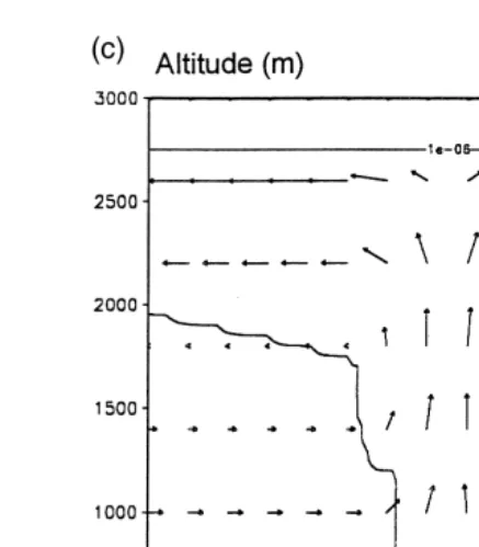
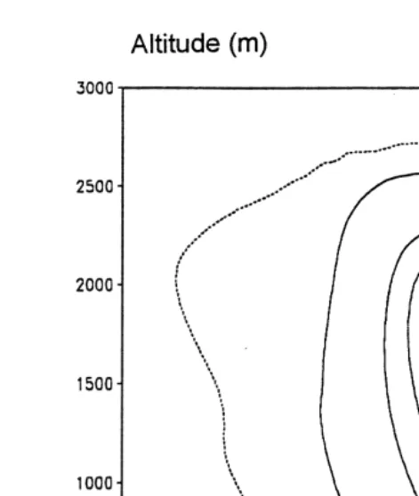
Fig. 1. Idealized flow field at three key times in the simulation. When radar reflectivity reachesy20 dBZ a ,
Ž .
and when the maximum updraft speed and the maximum radar reflectivity are attained b and c, respectively .
Ž y6 y1.
Cloud boundaries have been superimposed Qcs10 gg .
< Ž .<
where DV Õ ,Õ denotes the absolute value of terminal velocity difference between
t x y
raindrops with volumes Õ and Õ .
x y
Self-collection is treated in a way similar to that applied for accretion. The reduction rate for the raindrop number concentration is evaluated as a function of the mean
Ž .
volume drop radius, pre-computing and tabulating numerical solutions of Eq. 17 . The tendency equation for N isr
0 .5 2
<
d Nrrd tSFCs yN Cr
Ž
Õfr. Ž
r0rr.
Ž
18.
where the value of C is determined by linear interpolation on the logarithms of Õr. Ž .
The collisional break-up is taken into account by introducing a factor in Eq. 18 related to the coalescence efficiency of the most frequently colliding drop pairs. This factor is a function of the mean volume raindrop radius and its expression is identical to
Ž .
that used by Ziegler 1985 .
2.2. Vapor diffusion
2.2.1. Condensation of water droplet
The tendency equation for Q due to condensation is obtained integrating the massc
rate of change of a single drop over the cloud spectrum. The latter diffusional growth rate equation can be expressed as
where
y1
FTs
LvrKT L TŽ
v rRvy1.
q1rŽ
DvrsŽ .
T4
,FV is the ventilation factor, S is the supersaturation, r the drop radius, K the coefficient of thermal conductivity of air, L the latent heat of evaporation, R the gas constant forv v water vapor, D the diffusivity of water vapor in air,v rs the density of water vapor at saturation, and T the temperature.
Ž .
For cloud droplets the ventilation effect can be neglected FVs1 , therefore the
Ž . Ž .
integral value of Eq. 19 over the cloud spectrum can be easily obtained using Eq. 3 . Although, as an explicit condensation rate equation requires very small time steps, the
Ž .
semi-implicit procedure of Soong and Ogura 1973 is used to approximate the supersaturation in the resulting expression, taking into account the decrease in the water
Ž .
vapor mixing ratio and the attendant increase in saturation mixing ratio .
2.2.2. Nucleation
The cloud droplet number concentration is modified when condensation rate is insufficient to maintain exact saturation or when new cloud is forming. A log–linear
Ž U.
relation between the number of activated cloud condensation nuclei Nn and the locally steady supersaturation is assumed. The change in N due to nucleation is determinedc
evaluating NnU and comparing it with the cumulative number of activated cloud
Ž .
condensation nuclei previously processed by the parcel N , that is explicitly accounted.n
< < U
d Ncrd t NU Csd Nnrd t NUCsmax 0, N
Ž
n yNn.
rDt4
Ž
20.
The relation between NnU and S, suggested by the observers for this case, is given in
Ž .
In a subsaturated ambient, the cloud droplets are assumed to evaporate instantly. The decrease in the cloud number concentration due to evaporation, corresponding to the
Ž
mean droplet volume, is considered as a decrease in the number of activated nuclei see
Ž ..
Eq. 8 .
In the case of raindrops, the integral expression used to evaluate evaporation is
Ž . Ž .
obtained using Eqs. 3 and 19 , although the enhancement of vapor diffusion
associ-Ž
ated to ventilation cannot be neglected expressions for FV were those used by Hall,
.
1980 .
The traditional explicit equation for drop growth rate approximates the saturation
Ž .
vapor density rs with a linear function of the temperature difference between the drop and ambient air, when solving simultaneously the diffusion equations for water vapor
Ž .
Fig. 2. Time vertical section of simulated radar reflectivities. Abscissa indicates minutes after time 17:00 UTC.
this approximation. They proposed a more accurate explicit equation based on a second order approach that can be expressed as
w
d mrd tx
2sw
d mrd tx w
1 1yaSx
Ž
22.
w Ž .x Y X X
whereas1r2gr1qg rsrr rs srrs, the primes denote differentiation with respect to T, andgsL Dv rKrXs.
This expression that relates the first and second order approaches is then used as a correction factor in the rain evaporation integral expression. However, it introduces a negligible change for this case in which little evaporation occurs below cloud base.
2.3. Sedimentation
Rain number concentration and mixing ratio are independently sedimentated evaluat-ing the number and mass fluxes with the mean and mean mass terminal velocities, respectively. These mean terminal speeds are numerically evaluated using the Uplinger
Ž1981 expression that gives V as a function of the drop diameter D is. t Ž .
0 .5
w
x
3. Results
A comparison between observed and simulated characteristics of a convective cell is made using a kinematic reconstruction based on dual-Doppler data that corresponds to a summertime Hawaiian rainband occurred on August 10, 1990. This idealized flow field simulates the evolution of the updraft in magnitude and tilt. In Fig. 1a, b and c, the velocity field is shown for three key times, when the radar echo first appears, when the maximum updraft speed is attained and when the maximum radar reflectivity occurs.
Ž .
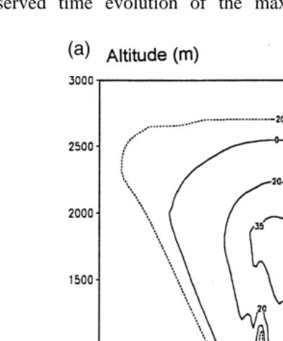
Extremely high radar reflectivities 59.7 dBZ have been observed within this cloud with a depth lower than 3000 m. The times required for the high reflectivity core to develop
Ž .
from an echo free region y20 dBZ up to 50 dBZ and its maximum value were 15 and 20 min, respectively. This echo free region was located in the middle of the cloud at an altitude of approximately 1700 m and the velocity field corresponds to that of Fig. 1a. A time-vertical section of the simulated radar reflectivity is shown in Fig. 2. The times taken for Z to reach 50 dBZ and its maximum from the value ofy20 dBZ, are very similar to those observed. The maximum of Z remains located at about 1700 m of altitude as the largest drops are suspended, until a strong vertical gradient associated
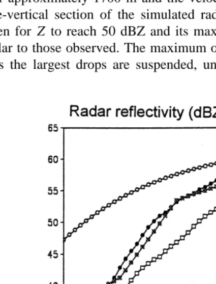
Fig. 3. Comparison between observed and simulated intensities of the maximum Z for the August 10 cell between 17:21 and 17:46 UTC. Closed squares correspond to the observed evolution. Open circles, open squares and closed circles correspond to simulated evolutions using a one-moment, two-moment schemes
0 2 Ž .
with the regions of most intense drop growth develops near the top of the cloud. In Fig. 3, the observed time evolution of the maximum Z during the stage of intense
Ž . Ž . Ž .
development is compared to those simulated using different schemes. Simulated curves are superimposed making approximate updraft maximum times coincident. It can be seen that the two-moment scheme performs better in simulating the evolution when
<
d Nrrd t AU T is evaluated preserving the second moment of the raindrop volume
distribu-Ž
tion rather than strictly preserving N . If a one-moment parameterization is applied thatr
.
used by Lin et al., 1986 and by Nicolini and Paegle, 1989 , the radar reflectivity
Ž .
evolution is much faster and a significantly higher value 63.4 dBZ is obtained for the maximum of Z, probably related to the overestimation of accretion rates and the concentration of large drops in Marshall–Palmer distribution.
From the beginning to the end of the simulation, the resulting Z fields exhibit a nearly symmetrical pattern and the maximum values of Z are located within the updraft core. The simulated Z fields begin to show a sloped pattern associated with the strong
Ž
divergence near the inversion level by the time vertical velocity is maximum see Fig.
.
1b . This pattern forms because the smaller the raindrop is, the farther it is carried outward from the updraft core and the slower it falls. The sloped base of this overhang first deepens downward with time and finally vanishes as the raindrops within it fell toward the surface, leading to an overall increase in the width of the cell. The simulated
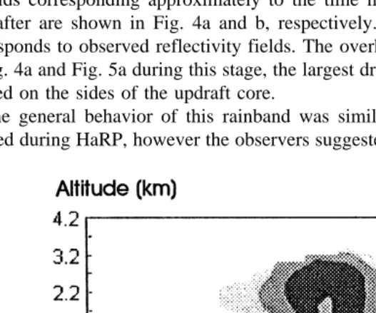
Z fields corresponding approximately to the time maximum updraft is attained and 5
min after are shown in Fig. 4a and b, respectively. Fig. 5 is analogous to Fig. 4 but corresponds to observed reflectivity fields. The overhang surrounding the cell is visible in Fig. 4a and Fig. 5a during this stage, the largest drops, associated to the overhang, are located on the sides of the updraft core.
The general behavior of this rainband was similar to those of several cases docu-mented during HaRP, however the observers suggested a parallel between this cell and a
Ž .
rainband occurred on July 23, 1985. Its time evolution, spatial dimensions and calculated reflectivities within the rainshaft corresponded closely to the features observed with
Ž .
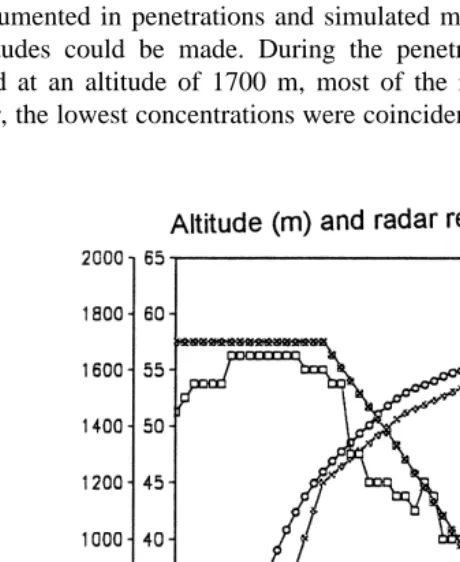
radar in the August 10 high reflectivity core Szumowski et al., 1998b , and their soundings and heights of inversion base were very similar. They performed several penetrations of this latter cell, each pass was targeted through the region of highest reflectivity using an on-board radar documenting the evolution of their high reflectivity core, drop spectra, as well as liquid water content and vertical velocity. The time evolutions of the calculated maximum Z and its observed altitude for this cell are shown in Fig. 6 and compared to simulated values. The July 23 sounding was used in this case and the simulated curves are superimposed making updraft maximum times coincident. There is a fairly good correspondence between the evolutions and positions of the observed and simulated cores. As a result, a comparison between microphysical informa-tion documented in penetrainforma-tions and simulated magnitudes for the corresponding times and altitudes could be made. During the penetrations at which the reflectivity core remained at an altitude of 1700 m, most of the raindrops were smaller than 1 mm in diameter, the lowest concentrations were coincident with the updraft core and the largest
drops were located on the sides. Those two maxima, associated to the overhang, were observed until 16:28. After this time, the largest raindrops were confined to narrower
Ž
regions located at the center of the updraft, as the core descended 0.3 km for the time at
.
which maximum Z occurred .
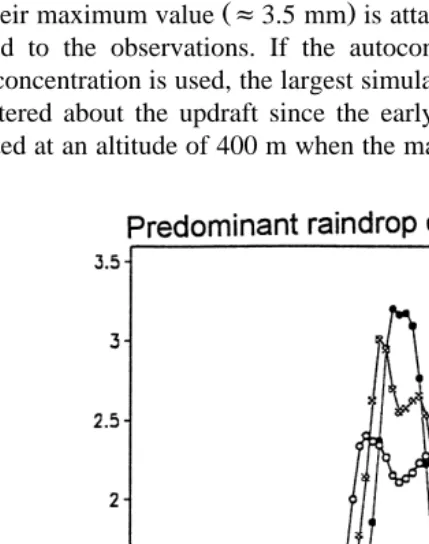
In Fig. 7, cross-sections of simulated predominant raindrop diameters are shown for altitudes of 1700, 1300, 900 and 400 m, and the corresponding times 16:23, 16:28,
Ž .
16:30 and 17:33 passes 2, 5, 6 and 7, see Szumowski et al., 1998b . The first curve, that is considered representative of the early stage in which drops are suspended at an altitude of 1700 m, begins to show two maxima located on the sides of the updraft core and those drops grow as the base of the overhang descends. The largest drops tend to be located at the updraft center as those drops, previously suspended, fall through the nearly vertical decaying updraft associated with the highest liquid water content. Largest
Ž
simulated predominant diameters are concentrated in a very narrow region less than 500
. Ž .
m and their maximum value f3.5 mm is attained at the time and altitude that closely correspond to the observations. If the autoconversion scheme that strictly preserves raindrop concentration is used, the largest simulated diameters are smaller and tend to be
Ž .
more centered about the updraft since the early stages not shown . Giant drops were
Ž
documented at an altitude of 400 m when the maximum value of Z occurred one of 8.2
.
mm in diameter , although drops of approximately 4 mm prevailed. Szumowski et al.
Ž1997, 1998b related the presence of these large drops, that grow by accretion as they.
fall through the decaying updraft with occurrence of extremely high radar reflectivities in summertime Hawaiian rainbands.
4. Conclusions
Even when the accuracy of a parameterized scheme could not be compared with those that explicitly solve the stochastic collection equation, for this case, it describes in a satisfactory manner the time required for the high reflectivity core to develop and some general characteristics of the cell evolution.
Results suggest that the typical overestimation of autoconversion and accretion in one-moment parameterized schemes is reduced by the presented two-moment one, showing a much better behavior. The evaluation of time rate of change of N due tor
autoconversion in terms of the corresponding rates for the first and second moments of the raindrop volume distribution, enhances the performance in simulating radar reflectiv-ities.
As simplicity is highly desirable when computer resources are rather limited, this warm rain scheme will be included, as well as the multimoment ice phase package under development, in the 2D non-hydrostatic convective cloud model of Nicolini and Paegle
Ž1989 . The above-mentioned model operates at the present with a one moment.
complete microphysics scheme.
Acknowledgements
The authors wish to thank the Consejo Nacional de Investigaciones Cientıficas y
´
Ž . Ž
Tecnologicas PIP 4526796 , the Agencia de Promocion Cientıfica y Tecnologica PICT
´
´
´
´
. Ž .
97 N 01757 and the University of Buenos Aires TX30 , for financial support.
References
Beheng, K., 1994. A parameterization of warm cloud conversion processes. Atmos. Res. 33, 193–206. Berry, E.X., Reinhardt, R.L., 1974. An analysis of cloud drop growth by collection: Part II. Single initial
distributions. J. Atmos. Sci. 31, 1825–1831.
Carrio, G.G., Levi, L., 1995. On the parameterization of autoconversion. Effect of small-scale turbulent´
motions. Atmos. Res. 38, 21–27.
Feingold, G., Levin, Z., Tzivion, S., 1991. The evolution of raindrop spectra: Part III. Downdraft generation in an axisymmetrical rainshaft model. J. Atmos. Sci. 48, 315–330.
Ferrier, B.S., 1994. A double moment multiple-phase four-class bulk ice scheme: Part 1. Description. J. Atmos. Sci. 51, 249–280.
Hall, W.D., 1980. A detailed microphysical model within a two-dimensional dynamic framework: model description and preliminary results. J. Atmos. Sci. 37, 2486–2507.
Kogan, Y.L., 1991. The simulation of a convective cloud in a 3-D model with explicit microphysics: Part I. Model description and sensitivity experiments. J. Atmos. Sci. 48, 1160–1189.
Lin, Y., Farley, R., Orville, H., 1986. Bulk parameterization of the snow field in a cloud model. J. Atmos. Sci. 22, 1065–1092.
Long, A.B., 1974. Solutions to the droplet collection equation for polynomial kernels. J. Atmos. Sci. 31, 1040–1052.
Meyers, M.P., Walko, R.L., Harrington, J.Y., Cotton, W.R., 1997. New RAMS cloud microphysics parameter-ization: Part II. The two-moment scheme. Atmos. Res. 45, 3–39.
Nicolini, M., Paegle, J., 1989. Real data deterministic forecasts of ambient motion fields upon convective precipitation. Second Int. Cloud Modeling WorkshoprConf. Toulouse, France, WMOrTD-No. 268, pp. 207–220.
Soong, S., Ogura, Y., 1973. A comparison between axisymmetric and slab-symmetric cumulus cloud models. J. Atmos. Sci. 30, 879–893.
Srivastava, R.C., Coen, J.L., 1992. New explicit equations for accurate calculation of the growth and evaporation of hydrometeors diffusion of water vapor. J. Atmos. Sci. 49, 1643–1651.
Szumowski, M.J., Rauber, R.M., Ochs, H.T., Beard, K.V., 1997. The microphysical structure and evolution of Hawaiian Rainband Clouds: Part I. Radar observations of rainbands containing high reflectivity cores. J. Atmos. Sci. 54, 369–385.
Szumowski, M., Grabowki, W.W., Ochs, H.T., 1998a. A simple two-dimensional kinematic framework designed to test warm rain microphysical models. Atmos. Res. 45, 299–326.
Szumowski, M.J., Rauber, R.M., Ochs, H.T., Beard, K.V., 1998b. The microphysical structure and evolution of Hawaiian Rainband Clouds: Part II. Microphysical measurements within rainbands containing high reflectivity cores. J. Atmos. Sci. 55, 208–226.
Uplinger, W.G., 1981. A new formula for terminal velocity. Proc. 20th Conf. on Radar Meteorology, Boston, Am. Meteor. Soc., pp. 389–391.
Walko, R.L., Cotton, W.R., Meyers, M.P., Harrington, J.Y., 1995. New RAMS cloud microphysics parameter-ization: Part 1. The single-moment scheme. Atmos. Res. 38, 29–62.