AUTOMATED RECONSTRUCTION OF WALLS FROM AIRBORNE LIDAR DATA FOR
COMPLETE 3D BUILDING MODELLING
Yuxiang He*, Chunsun Zhang, Mohammad Awrangjeb, Clive S. Fraser
Cooperative Research Centre for Spatial Information, Department of Infrastructure Engineering University of Melbourne, VIC 3010, Australia
[email protected], (chunsunz, mawr, c.fraser)@unimelb.edu.au
Commission III, WG III/2
KEY WORDS: LIDAR, Three-dimensional, Principle Component Analysis, Segmentation, Feature extraction, Vertical wall
ABSTRACT:
Automated 3D building model generation continues to attract research interests in photogrammetry and computer vision. Airborne Light Detection and Ranging (LIDAR) data with increasing point density and accuracy has been recognized as a valuable source for automated 3D building reconstruction. While considerable achievements have been made in roof extraction, limited research has been carried out in modelling and reconstruction of walls, which constitute important components of a full building model. Low point density and irregular point distribution of LIDAR observations on vertical walls render this task complex. This paper develops a novel approach for wall reconstruction from airborne LIDAR data. The developed method commences with point cloud segmentation using a region growing approach. Seed points for planar segments are selected through principle component analysis, and points in the neighbourhood are collected and examined to form planar segments. Afterwards, segment-based classification is performed to identify roofs, walls and planar ground surfaces. For walls with sparse LIDAR observations, a search is conducted in the neighbourhood of each individual roof segment to collect wall points, and the walls are then reconstructed using geometrical and topological constraints. Finally, walls which were not illuminated by the LIDAR sensor are determined via both reconstructed roof data and neighbouring walls. This leads to the generation of topologically consistent and geometrically accurate and complete 3D building models. Experiments have been conducted in two test sites in the Netherlands and Australia to evaluate the performance of the proposed method. Results show that planar segments can be reliably extracted in the two reported test sites, which have different point density, and the building walls can be correctly reconstructed if the walls are illuminated by the LIDAR sensor.
1. INTRODUCTION
Digital building models are required in many geo-information applications. Airborne Light Detection and Ranging (LIDAR) has become a major source of data for automated building reconstruction (Vosselman, 1999; Rottensteiner and Briese, 2002; Awrangjeb et al., 2010). With its increasing density and accuracy, point cloud data obtained from airborne LIDAR systems offers ever greater potential for extraction topographic objects, including buildings, in even more detail. While considerable achievements have been made in building roof extraction from airborne LIDAR, limited research into the modelling and 3D reconstruction of vertical walls has thus far been carried out. However, walls are important components of a full building model, and without walls a building model is incomplete and potentially deficient in required modelling detail. Yet, in certain applications such as car and personal navigation, building walls are more important than roofs in city models.
The main difficulty for wall reconstruction is the typical low density and irregular distribution of LIDAR points on vertical façades. In this paper a method for automated extraction and reconstruction of vertical walls from airborne LIDAR data is presented. The automated identification and location of wall points, along with the development of new methods for reliable segmentation and classification of point clouds has formed the focus of the reported research. These developments are detailed in Section 3, together with approaches for wall reconstruction and modelling. Two test sites have been employed to evaluate the developed algorithms and experimental results are presented
in Section 4. A discussion of the developed approach is presented in Section 5, along with concluding remarks.
2. RELATED WORK
Automated building reconstruction from airborne LIDAR data has been an active research topic for more than a decade (Vosselman and Dijkman, 2001). Since buildings are usually composed of generally homogeneous planar or near-planar surfaces (Hug, 1997; Oude Elberink, 2008), significant efforts have been directed towards the development of algorithms for automated point cloud segmentation of planar surfaces. For example, building roofs are generally reconstructed by exploring the spatial and topological relations between planar roof segments.
Segments can be determined by region growing methods, using edge-based approaches, or via clustering techniques. Region growing approaches start with a selected seed point, calculate its properties, and compare them with adjacent points based on certain connectivity measurement to form the region. Vosselman and Dijkman (2001) explored the use of Hough Transforms for planar surface detection. A random point and its certain neighbours were first selected and transformed into 3D Hough space. The point was then adopted as a seed point in the case where all the neighbours in Hough space intersected into one point. The other strategy of seed selection is RANSAC (Brenner, 2000; Schnabel et al., 2007). A comparison of the two strategies has been reported by Tarsha-Kurdi et al. (2007). Normal vectors from neighbouring points also provide crucial information for segmentation. Sampath and Shan (2010) International Archives of the Photogrammetry, Remote Sensing and Spatial Information Sciences, Volume XXXIX-B3, 2012
performed clustering based on normal vectors by applying the k-Means algorithm and then extending the clusters to the edge points to form segments while Kim and Medioni (2011) used a hierarchical approach to cluster normals. Bae et al. (2007) used an edge detection approach for segmentation where local curvature was employed for detection of edges. Level set approaches have also been used for curve propagation and segmentation (Kim and Shan, 2011).
Vertical wall extraction is attractive to some applications. Oude Elberink (2008) compared positional differences between roof outline and ground plans. The result showed that a 3D building model can generally not be correctly formed by simply projecting roof edges to the ground to form the vertical walls. However, very limited efforts have been made so far to explicitly derive building walls from airborne LIDAR data. Dorninger and Nothegger (2007) introduced data mining approach for clustering wall seeds in feature space. Rutzinger et al. (2009) used a Hough transform segmentation algorithm for extracting walls from both airborne and terrestrial mobile LIDAR data and compared the accuracy of the two dataset. Currently, mobile LIDAR data is being widely used for vertical walls reconstruction (Hammoudi et al., 2010; Rottensteiner, 2010).
3. METHODOLOGY
The proposed approach for wall detection and reconstruction consists of three stages, as indicated in Figure 1. One of the main requirements of the developed method is automated identification and location of wall points via improved point cloud segmentation and classification. Following this stage, wall surfaces are formed. The walls are then reconstructed and their extents and corners are determined through geometrical and topological modelling that is constrained by roof structure.
Figure 1. Workflow of the proposed methodology.
3.1 Segmentation
The developed point cloud segmentation approach follows the region growing principle. The major contributions of the presented work include optimal determination of search range and robust selection of seed points. In the approaches of region growing, the selection of seed points and the determination of the search radius are critical (Brenner, 2000; Vosselman and Dijkman, 2001). Randomly selected seed points may result in incorrect results or too many unnecessary small segments. A larger search range may pick up points outside the segments under consideration. A smaller search range seems safe, but it may miss points, particularly when the density of the point cloud is low or the distribution of the points is irregular. To avoid such problems, an approach to adaptively determine the search neighbour from the point cloud has been developed. The search range varies according to the local density and distribution, and it increases with low density. In addition, the selection of seed points is determined via a Principle Component Analysis (PCA) process. Only the points that exhibit high planarity in a local area are selected.
Adaptive neighbourhood searching. Either k-Nearest or Fixed Radius method, or combination of both, is generally employed for searching for neighbouring points. These methods work well when the point distribution is regular. However, their
performance can be poor when point density varies (Rutzinger et al., 2009). In this paper, adaptive method is developed to accommodate point distributions and decide suitable neighbourhoods.
Let D p |i 1, n be whole point cloud with n points and
p D be the point whose neighbourhood is to be decided. Firstly, a set of k-nearest points from is determined. Then, the largest distance between and in can be determined among its k neighbours:
d arg max #distance#p,p (( , i = 1,2,...,k (1)
To optimal the neighbourhood selection scale, dynamically scale r is then decided as ) d /3 (Pauly 2002) and thus the neighbours of can be represented as
N -p./p. N0, distance1p.,p 2 3 )4 (2)
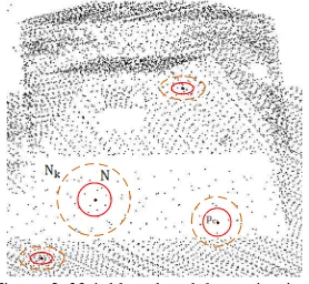
Thus, the neighbour N ensures the uniformly of neighbourhood distribution and optimal search range. Figure 2 shows four cases of neighbourhood determination. The dashed circles represent the range of the k-nearest points. The determined neighbours are shown in circles of solid circles. The LIDAR point densities on roofs and the ground are high and the distribution of the points demonstrates a quite regular pattern. Therefore, the search ranges on the roof and the ground are similar and small. Wall points are sparse and the distribution varies with the flight line and scanning directions, so a larger search ranges is adapted. An interesting performance is seen near the intersection of wall and ground, as shown in the lower right of Figure 2. The k-nearest or fixed radius methods may result in a large amount of ground points (see the dashed circle). This kind problem can be avoided by the proposed adaptive search range approach (see the solid circle).
Figure 2. Neighbourhood determination.
Local surface variation. A planar surface can be estimated within the determined neighbourhood and its planarity can be assessed by PCA. The PCA of a set of 3D LIDAR points yields the principal vectors describing an orthonormal frame (v0, v1, v2)
and the principal values (56, 57, 58) with 56<57< 58. The PCA
decomposition of a set of LIDAR points can be calculated by singular value decomposition of the 3 9 3 covariance matrix of the points. The covariance of :and :; is defined as
cov1X , X.2 ∑ #@ABµA(1@DBµD2
E F
GB7 (3)
Here, µ denote the mean of X, and n is the number of LIDAR points in the neighbourhood.
For planar points, the variances will appear only in two orthogonal directions after PCA transformation. That is, λ6 is
zero. Thus, we define local surface variation index (IJKL) based on the principal values is defined as
IJKL# ( MNO MMNFOMP (4) reported in (Hoppe et al., 1992; Sampath and Shan, 2010).
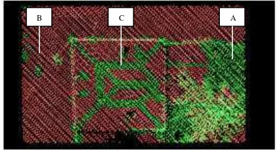
An example of PCA process is given in Figure 3. The scene consists of an independent house with vegetation on its left side. The vegetation points with discontinuous surfaces, in green in Figure 3(A), tend to be non-planar points. The bare-earth is relatively flat and points on this surface, indicated in red in Figure 3(B), are determined as planar. The roof of this house constitutes several planes joined by roof ridges. While most roof points are planar, points on ridges, shown in Figure 3(C) are not. They are successfully differentiated from the plane points by the PCA process.
Figure 3. Results of PCA process of LIDAR points (green points are non-planar while red ones is planar)
Seed points are then selected from the determined planar points. However, not all planar points are suitable candidates. For instance, a vegetation point with only a few neighbouring points may have a very low IJKL value. In order to avoid such vegetation points, only the planar points with a certain size of neighbourhoods are considered as valid seed points.
Region growing for segmentation. The coordinates for a seed point, along with the local surface normal (v0 determined in the
PCA process), define the initial plane. Then, the neighbourhood of the seed point is examined and the distances of the neighbouring points to the plane are computed. A neighbouring point is considered belonging to the plane if its distance to the iterative process will collect points to build up the plane. Some regions like gable roofs, points are over-segmented by multiple segments. In such case, the normal direction of over-segmented point is used to compare with the segments and group into the segment with most homogeneous.
3.2 Segment classification
The detected segments undergo classification so that object features such as roofs, walls and ground surface are
differentiated within the LIDAR point cloud. Firstly, walls are identified based on the segment normal vectors. Since walls are vertical, the Z-component of the segment normal vector should be zero. The remaining segments will be processed to derive roofs and ground surfaces. Common knowledge used in classification is that roofs are above the ground and connect with it via vertical walls; and if a wall is not presented in LIDAR data, there will be a large height jump between the roof segment and the ground segment. The height different between two segments is defined as nearest distance of two groups of point cloud and from the pair of nearest points to derive height jump. The classification is then carried out by the following segment is on top of the wall, it is classified as roof. Also, if a vertical wall does not appear in the neighbourhood, but this segment displays a significant height jump compared to its neighbours, it will again be classified as roof. The segment is then removed from the list and Step 2 is repeated. If the highest segment has small height difference with its neighbours, merge this segment with its neighbours and update the list. Then repeat from step 2. 4. If the highest segment has small height difference from its
neighbours, it is merged with them and the list is updated. The process from Step 2 is then repeated.
5. The above procedure is iteratively repeated until all roof segments and wall segments are identified.
6. The remaining segments are taken as ground surface.
3.3 Reconstruction of walls
With the extracted wall segments, the reconstruction of walls is straightforward. It is worth to note that some wall points may not be collected in the wall segments due to the sparse distribution and irregular pattern of LIDAR illumination on building walls. Since walls are between roofs and ground, these wall points can be located from the neighbourhood of the roof determined by topological and geometrical modelling using roof structure information.
Firstly, the roof segment on top of the wall plane is located. The horizontal plane passing through the roof edge is actually the eaves of the roof segment. The intersection of eaves with the fitted wall plane leads to the top outline of the wall. Wall corners are usually located under the roof ridge and the intersection of the wall plane, eave and roof ridge generate wall corners.
4. EXPERIMENTAL TESTS AND RESULTS
The developed algorithms have been tested with a number of datasets for different urban scenes in Europe and Australia. Here, results from two test sites will be presented. The first test area is located in Enschede, The Netherlands. The scene is flat. As in many European towns, the scene includes free-standing low residential buildings, as well as streets and trees. Data was acquired by FLI-MAP 400 with 20 pts/m². The high density of
A
B C
the point cloud was achieved by fusion of several flights. This has introduced inconsistency in the dataset.
The second test site is part of the campus of the University of Melbourne, Australia. The data was collected in a recent campaign by Optech ALTM Gemini with 4-5 pts/m². The scene contains larger buildings. Due to low density of the point cloud, only a few building walls were illuminated by the LIDAR sensor.
4.1 Parameter setting
Adaptive scale factor for searching neighbours is mainly depended on the initial k selection. Due to the final scale factor is three times less than initial scale factor, the searching region is nine times less than initial one. Initial k is estimated based on point density and visual inspection for two datasets and selected as 90 and 40 empirically.
Ideally, the local surface variation index should be zero for a planar point. Thus, a small value can be assigned as the threshold. Figure 4 shows the results of a portion of the Enschede dataset with threshold values (IJKL) of 0.005, 0.01, 0.015 and 0.02 respectively. It can be seen roof points were largely misclassified with 0.005 and 0.01. This is because the point cloud was a fusion of several acquisitions with discrepancies (up to 3-6 cm by manual inspection). A larger value of the threshold can account for the quality of such data, as shown in the results using 0.015 and 0.02 as the threshold. However, the result of value 0.02 led to misclassification of vegetation points as planar points. Therefore, the optimal threshold has been set to 0.015 in the reported testing.
Figure 4. Detected planar points using threshold of 0.005 (a), 0.01 (b), 0.015 (c) and 0.02 (d) for local surface variation index. Red indicates planar points while green for non-planar points.
To set an appropriate tolerance value QV for segment generation, four training samples of flat surface were selected from the Enschede dataset. The standard deviations of these four sites were calculated and listed in Table 1.
Flat site 1 2 3 4
Standard
deviation (m) 0.053 0.032 0.046 0.064
Number of
points 1446 2462 2711 804
Table 1. Standard deviations of flat plane
Sites 1 and 4 were captured in multiple flight lines and thus have larger standard deviation. A confidence interval of 2X was defined as the tolerance. Taking the sample size and the RMS into account, the tolerance distance value for the Enschede data
was set to 0.09 m. A similar procedure was applied to the Melbourne dataset, and the optimal local surface variation and tolerance distance toward plane as 0.02 and 0.10m, respectively, were selected.
4.2 Verification
Correctness as well as completeness for verification of extraction result was performed by manually outlined building facades from point clouds. A buffer from reference wall facades was preformed for evaluating correctness and completeness. The correctness was calculated as the length of the extracted lines inside the buffer divided by the length of all extracted lines. The completeness was defined as the length of the extracted lines inside the buffer divided by the length of the reference lines. The width of buffer is selected as 40cm which we believe the true position of wall facade should inside in this research.
Site 1 2
Correctness 0.75 0.65
Completeness 0.62 0.32
Table 2. Correctness and completeness of verification
4.3 Result of wall reconstruction
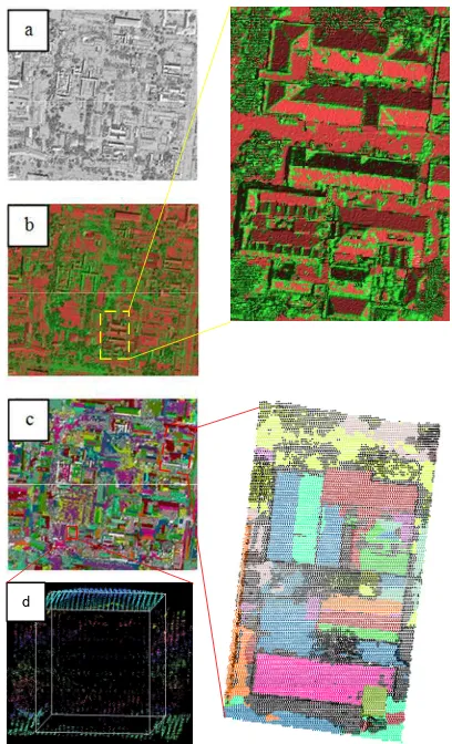
The datasets were processed with the methods described in the previous section. A portion of raw point cloud of the Enschede data is shown in Figure 5. The seed points were extracted and the segments were coded by colours. It can be seen that the building roofs were successfully extracted as planar segments while the vegetation points were treated as non-planar (shown in white in the Figure 5). Since the site in Enschede is quite flat, the ground surface was also clustered into several large planar patches. The detected walls are presented in Figure 6. On the left of the figure, walls are shown in 2D while the 3D wall facades are shown on the right. Some gaps exist in wall facades. This is caused by absence of LIDAR points. It was also noticed that a few small facades were detected in vegetation area. These false detections can be removed easily due to their sizes are small.
Figure 5. Segmentation result in Enschede site. (non-segmented points are represented in white)
Figure 6. Extracted wall facades in the Enschede data.
a b
c d
Finally, the wall façades were modelled using the information of building roof structures. The roof segments, eaves and roof ridges were explored to determine the wall extent and corners. Several examples are given in Figure 7. The initial wall outlines in Figure 7(b) were derived by detected wall points. Initial outlines were incomplete and incorrect. After modelling using building roof structure information, the wall boundary and corners were determined in Figure 7(c). The 3D models of the full buildings are shown in Figure 7(d).
(a) (b) (c) (d) Figure 7. Detection of cubic buildings. (a) point cloud of
original building; (b) detected wall outlines; (c) constraint wall outlines; (d) wall façade cubes
d
Figure 8. Result of Melbourne campus site. (a) raw data, (b) detected planar points (red) and non-planar points (green), (c) generated segments, (d) reconstructed walls.
The wall reconstruction performance for the Melbourne data is shown in Figure 8. The algorithms worked equally well, even considering that the point density was lower than in the Enschede data. Once again, the planar points (roof points, terrain points) and non-planar points (vegetation points, roof ridge points) were successfully detected, as indicated in Figure 8(b). Planar segments, including roof façades and ground surfaces were derived by region growing using the planar seed points, as seen in Figure 8(c). Although only a small number of walls were illuminated by the LIDAR sensor due to the flight pattern, these walls were successfully extracted. An example of reconstructed walls is shown in Figure 8(d).
5. DISCUSSIONS AND CONCLUSIONS
This paper has presented a methodology for automated reconstruction of building walls from airborne LIDAR data. All procedures have been detailed, including point cloud segmentation and classification, wall reconstruction and modelling. The developed approaches have been tested using different datasets. Experimental results are presented.
Segmentation plays a critical role in point cloud processing, particularly for object reconstruction. To achieve high quality segmentation, new approaches to search range determination and seed point selection have been proposed and implemented. Adaptive determination of search range can efficiently accommodate varying point cloud densities. Results show that PCA is an effective method to select planar points for segmentation. Thus, non-planar points, such as vegetation points, can be avoided from beginning. In both test sites, in Europe and Australia, all the roof segments, wall segments and planar ground segments were correctly extracted and modelled from the LIDAR point cloud, even though the point density was very different in each case. Thus, the developed segmentation method can be also used for roof reconstruction and terrain extraction. This method may also be applicable for tree detection upon further refinement.
The experiments conducted have also shown that the wall plane can be determined from LIDAR points. However, LIDAR points alone are not sufficient to decide the wall boundaries. The extent and corners of extracted wall planes can be reconstructed with geometrical and topological relations between the wall and the roof structures. This modelling process proved to be powerful. Verification of correctness and completeness is preformed. Even though correctness is relatively higher than completeness, both are low due to point distribution.
The reconstructed walls together with the 3D roofs generate complete 3D building models. Unfortunately, many walls cannot be reconstructed from the LIDAR point cloud since they are not ‘seen’ by the sensor. With the decreasing cost of airborne LIDAR, oblique scanning for dense wall point cloud coverage may well be more practical in the future.
The sensitive of parameter setting and accuracy of segmentation result should be further investigated. Future research will refine the method for wall reconstruction and in general for building reconstruction. For instance, the current method reconstructs roofs and walls separately. New approaches may be researched to more efficiently explore the inherent relationships between different parts of a building so as to generate comprehensive building models with simultaneous roof and wall extraction and modelling.
ACKOWLEDGEMENT
The presented work has been conducted under the support of the Cooperative Research Centre for Spatial Information. We thank Prof. G. Vosselman at ITC for allowing us to use the Enschede dataset for this research.
REFERENCES
Awrangjeb, M., Ravanbakhsh, M., Fraser, C., 2010. Automatic detection of residential buildings using LIDAR data and multispectral imagery. ISPRS Journal of Photogrammetry and Remote Sensing, 65(5), pp. 457-467.
Bae, K. -H., Belton, D., Lichti, D. D., 2007. Pre-processing procedures for raw point clouds from terrestrial laser scanners. Journal of spatial science, 52(2), pp. 65-74.
Brenner, C., 2000. Towards fully automated generation of city models. In: The International Archives of Photogrammetry, Remote Sensing and Spatial Information Sciences, 33, pp. 85-92.
Dorninger, P., Nothegger, C., 2007. 3D segmentation of unstructured point clouds for building modelling. In: The International Archives of Photogrammetry, Remote Sensing and Spatial Information Sciences, 35, pp. 191-196.
Hammoudi, K., Dornaika, F., Soheilian, B., Paparoditis, N., 2010. Extracting outlined planar clusters of street facades from 3D point clouds. In: IEEE Canadian Conference on Computer and Robot Vision, pp. 122-129.
He, Y., 2010, Segment - based Approach for Digital Terrain Model Derivation in Airborne Laser Scanning Data. M.Sc thesis, University of Twente Faculty of Geo-Information and Earth Observation (ITC), 63p.
Hoppe, H., DeRose, T., Duchamp, T., McDonald, J., Stuetzle W., 1992. Surface reconstruction from unorganized points. In: Computer Graphics (SIGGRAPH ’92), 26, pp. 71-78.
Hug, C., 1997. Extracting Artificial Surface Objects from Airborne Laser Scanner Data. In Grün, A., Baltsavias, E. P., and Henricson, O. (Eds.), Automatic extraction of man-made objects from aerial and spaceimages (II),Birkhäuser, Basel, pp. 203-212.
Kim, E., Medioni,G., Urban scene understanding from aerial and ground LIDAR data. Machine Vision and Application, 22(4), pp. 691-703.
Kim, K., Shan, J., 2011. Building roof modelling from airborne laser scanning data based on level set approach.ISPRS Journal of Photogrammetry and Remote Sensing, 66(4), pp. 484-497.
Levin, D., 2003. Mesh-independent surface interpolation. In Geometric Modeling for Scientific Visualization, pp. 37-49.
Oude Elberink, S., 2008. Problems in Automated Building Reconstruction based on Dense Airborne Laser Scanning Data. In: The International Archives of Photogrammetry, Remote Sensing and Spatial Information Sciences, 37, pp. 93-98.
Pauly M., Gross M., Kobbelt L.P., 2002. Efficient simplification of point-sampled surfaces. In Proceedings of the conference on Visualization ’02, pp.163–170.
Rottensteiner, F., 2010, Automation of object extraction from LIDAR in urban areas, In: IEEE International Geoscience and Remote Sensing Symposium, pp. 1343-1346.
Rottensteiner, F., Briese, C., 2002. A new method for building extraction in urban areas from high-resolution LIDAR data. In: The International Archives of Photogrammetry, Remote Sensing and Spatial Information Sciences, 34, pp. 295-301.
Rutzinger, M., Oude Elberink, S., Pu, S., Vosselman, G., 2009. Automatic extraction of vertical walls from mobile and airborne laser scanning data. In: The International Archives of Photogrammetry, Remote Sensing and Spatial Information Sciences, 38, pp. 7-11.
Sampath, A.; Shan, J., 2010. Segmentation and reconstruction of polyhedral building roofs from aerial LIDAR point clouds. IEEE Transactions on geosciences and remote sensing, 48(3), pp. 1554-1567.
Schnabel R., Wahl R., Klein R., 2007. Efficient RANSAC for pointcloud shape detection. In: Computer Graphics Forum, 26(2), pp. 214-226.
Tarsha-Kurdi F., Landes T., Grussenmeyer P., 2007. Hough-transform and extended RANSAC algorithms for automatic detection of 3d building roof planes from LIDAR data. In: The International Archives of Photogrammetry, Remote Sensing and Spatial Information Sciences, 36, pp. 407-412.
Vosselman, G., 1999. Building reconstruction using planar faces in very high density height data. In: The International Archives of Photogrammetry, Remote Sensing and Spatial Information Sciences, 32, pp. 87-92.
Vosselman, G., Dijkman, S., 2001. 3D Building Model Reconstruction from Point Clouds and Ground Plans. In: The International Archives of Photogrammetry, Remote Sensing and Spatial Information Sciences, 34, pp. 37-43.