The role of Ekman pumping and the dominance of swirl in confined flows driven by
Lorentz forces
P.A. Davidson *, D. Kinnear, R.J. Lingwood, D.J. Short, X. He
Department of Engineering, University of Cambridge, Trumpington Street, Cambridge, UK
(Received 23 November 1997; revised 30 August 1998; accepted 13 October 1998)
Abstract – We are concerned here with confined, axisymmetric flows of small viscosity driven by a prescribed Lorentz force. In a previous paper we examined the case where the body force is purely azimuthal, generating a swirling motion. We showed that, in such cases, Ekman pumping provides the means by which the flow establishes a steady state. In this paper we examine a problem which, superficially, looks rather different. That is, we consider the case where the dominant Lorentz force is poloidal(Fr,0, Fz)in(r, θ, z)coordinates, while the azimuthal component of force is taken to be small
but finite. This characterizes many important industrial processes and it is well known that such flows exhibit a curious phenomenon. That is, provided the azimuthal forcing exceeds a relatively low threshold (about one percent of the poloidal force), the flow is dominated, not by poloidal motion, but by swirl. Previous explanations of this phenomenon are inconsistent-with the experimental evidence. Here we offer an alternative view. We show that, once again, the pool dynamics are controlled by Ekman pumping, and that the dominance of swirl is a direct consequence of the suppression of the poloidal motion by the radial stratification of angular momentum.Elsevier, Paris
1. Introduction
1.1. The experimental evidence for the dominance of swirl
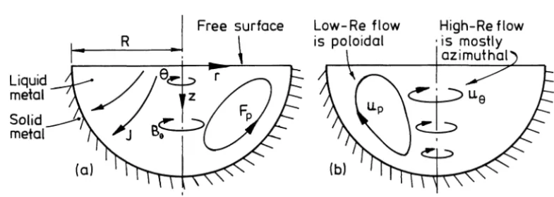
There is a well-known and mush reported experiment, first performed by Bojarevics, Millere and Chaikov-sky [1], which exhibits a curious phenomenon, often called swirl bifurcation. In this experiment current is passed radially downward through an axisymmetric pool of liquid metal, as indicated in figure 1. The interaction of the current density, J, with its associated magnetic field,Bθ, gives rise to a Lorentz force, F=J×B/ρ, which is poloidal ((Fr,0, Fz)in(r, θ, z)coordinates). Of course, the resulting motion is also poloidal; at least this is the case at low levels of forcing. At higher current levels, though, a surprising phenomenon is observed. The pool is seen to rotate, and this rotation is much more vigorous than the poloidal motion. Our aim is to explain this phenomenon.
In some sense, the observed rotation must result from a lack of symmetry in J or B. That is, a finite azimuthal force, Fθ, is required to maintain the swirl and in particular to overcome the frictional torque exerted on the pool by the boundaries. This additional force is thought to arise from the interaction of J with a weak, stray magnetic field. (For example, a vertical fieldBz gives rise to an azimuthal force−JrBz/ρ.) Nevertheless, it is surprising that a force composed of a large poloidal component plus a weaker azimuthal contribution can give rise to a flow dominated by swirl, i.e.uθ≫ur, uz. In the experiment of Bojarevics et al. the stray field arises in part from the earth’s magnetic field. At the lower levels of current used (∼15 Amps) the average magnetic field induced by the current on the pool surface is∼0.6 Gauss, which is comparable with the earth’s magnetic
Figure 1. Experiments of Bojarevics et al. (a) Current flows down through the pool of liquid metal and the interaction of J with its self magnetic field,
Bθ, produces a poloidal force, Fp. (b) At low levels of current the flow is poloidal, while higher levels of current initiates an intense swirling motion.
field. However, at the highest current levels (∼1200 Amps) the average surface value ofBθ is around 42 Gauss, which is a factor of∼100 greater than the earth’s magnetic field. The key question, therefore, is why do low levels of azimuthal forcing give rise to disproportionately high levels of swirl?
The same phenomenon is seen at a larger scale in industrial processes such as electric-arc and electro-slag remelting of ingots. Here current is fed into the pool across its entire top surface, and the stray magnetic field arises from inductors which carry current to and from the apparatus (Moreau [2]). Unless great effort is made to minimize the stray magnetic fields, unwanted swirling motion is generated in the pool.
In all of these examples the Reynolds number, Re, is high, perhaps 300–104 in Bojarevics experiment, and around 105 in industrial applications. It is likely, therefore, that most of these flows are turbulent. Moreover,
the phenomenon seems to be particular to high-Reynolds numbers, in the sense that there is a value of Re below which disproportionately high levels of swirl are not observed (Bojarevics et al. [1]). There is, however, a second threshold. That is, as we shall show,uθ dominates the poloidal motion, up, only when Fθ exceeds ∼0.001|Fp|. (We use subscriptpto indicate poloidal components of u or F.) Below this threshold, the poloidal motion remains dominant, no matter what the value of Re. In particular, ifFθ →0 then there is no swirling motion at all.
In summary, then, the term swirl bifurcation is commonly used to describe high-Re flows in which the forcing has both azimuthal and poloidal components, F=Fθ+Fp, but where the swirl dominates the motion despite the relative weakness of Fθ. That is,
uθ≫ |up|, Fθ≪ |Fp| (Re≫1). (1)
Note that it is not the appearance of abnormally high values ofuθ which typifies the experiment. Rather, it is the high values of the ratiouθ/|up|which is unexpected. This distinction may seem trivial, but we believe it is important. Some authors see this phenomenon as an instability, with the appearance of swirl being analogous to the sudden eruption of Taylor vortices is unstable Couette flow. Our view is different. We believe that the magnitude ofuθ is simply governed by the (prescribed) magnitude of Fθ, and that it is an unexpected suppression of|up|, rather than a growth inuθ, which typifies the observations.
1.2. Spontaneous rotation or poloidal suppression?
is not thatuθ is unexpectedly large, but that, in the presence of swirl,|up|is disproportionately small. In fact, the magnitude ofuθ can always be estimated from the global torque balance,
ρ Z
rFθdV =
I
2π r2τθds. (2)
Heres is a curvilinear coordinate measured along the pool boundary and τθ is the azimuthal surface shear stress. In a turbulent flowτθ =cf(1/2)ρu2θ where the skin friction coefficientcf is, perhaps, of the order 10−2 (Davidson, Short and Kinnear [3]). (Strictlycf is a function of Reynolds number, but in the range 103–105, cf ∼10−2. See Section 3.) IfRis a typical pool radius this yields the estimate
uθ∼(RFθ/cf)1/2∼10(RFθ)1/2. (3)
Similar estimates may be made for laminar flow (Davidson [4]) but the details are unimportant. The key point is thatuθ is fixed in magnitude byFθ.
Our primary thesis is that flows of type (1) arise from the action of the centrifugal force. That is, there are two potential driving forces for poloidal motion, the poloidal Lorentz force, Fp, and the centrifugal force −(u2θ/r)ˆer, and we shall see that these conspire to eliminate each other. Specifically, provided Re≫1 and Fθ/|Fp|>∼0.01, the angular momentum of the fluid always distributes itself in such a way that these two forces almost exactly cancel (to within the gradient of a scalar) and that consequently, the poloidal motion is extremely weak. We shall show that it is this balance between Fp andu2θ/rwhich underpins the experimental observations. Moreover, this phenomenon is not restricted to any particular distribution of current (such as the discharge from a point electrode), but is a general property of confined flows with combined azimuthal and poloidal forcing.
1.3. Conventional explanations of the dominance of swirl
Some authors attach great significance to the fact that there appears to be a threshold value of Re above which swirl is dominant. This has led them to conclude that the underlying poloidal motion is unstable and that the appearance of swirl is simply a manifestation of this instability. Consequently, it has been popular to study the breakdown of a well-known self-similar poloidal flow associated with the injection of current from a point source located on the surface of a semi-infinite domain. These studies are characterized by the fact that a Jeffery–Hamel-like solution to the point electrode problem breaks down at low values of Re, but that a self-similar solution may be re-established above the critical value of Re if (somehow) just the right amount of angular momentum is injected into the flow. (There is no azimuthal forcing in these problems.) One of the main conclusions of this type of analysis is that flows which converge at the surface are potentially unstable, whereas those which diverge are stable. (Self-similar diverging flows may be realized using a slightly more complex, but still singular, arrangement of current injection.) We believe that, while formally correct, these analyses are of little relevance to the experimental observations, which inevitably relate to finite domains and so are subject to the global constraint (2). The explanation of the experiment of Bojarevics et al. is, therefore, still an open question.
Figure 2. Geometry analysed by Shtern and Barrero [5]. Rather than consider a flat surface they investigated flows in a semi-infinite domain with a conical surface.
two crucial respects. First, as already noted, there is no outer frictional boundary and so their model problem is free from the integral constraint (2). That is, no external torque is required to maintain the swirl. Second, the streamlines in the self-similar solution do not close, but rather converge radially, as shown in figure 2. Now it happens that at Re∼5 the similarity solution breaks down in the sense that the velocity on the axis becomes infinite. However, if just the right amount of swirl is introduced into the far field then, due to the radially inward convection of angular momentum, the singularity on the axis is alleviated. Thus in semi-infinite domains there exists the possibility of a bifurcation from a non-swirling to a swirling flow, provided, of course, that (somewhat) nature provides just the right amount of angular momentum in the far field. This, according to the authors, is the origin of the experimental observations.
But there are several fundamental objections to making the jump from infinite to confined flows. The first point to note is that the Lorentz-driven flow in a hemisphere bears little resemblance to the self-similar flow in an infinite domain. Ifr0 is the pool radius and ri the electrode radius then a self-similar solution may be justified only in the small regionri≪(r2+z2)1/2≪r0. In the experiments of Bojarevics et al. no such region
exists(r0/ri∼45). Besides, the evidence for swirl bifurcation (or poloidal suppression as we prefer to call it) is not restricted to point sources of current, but rather exists for many different distributions of current within the pool (see Section 5). An explanation of this behaviour which rests on the breakdown of a very particular class of motion (the self-similar flow) cannot explain the widespread occurrence of this phenomenon. The second key point is that the model problem of Shtern and Barrero [5] relies on angular momentum being imposed in the far field. In confined domains where does this angular momentum come from? If swirl exists in confined flows it must be maintained by an external torque and the magnitude of this torque fixes the magnitude of the swirl. There can be no sudden “eruption” of swirl due to an increase in Re. Third, according to the Shtern and Barrero model, the sudden appearance of swirl occurs only if the flow converges at the surface. In practice, however, this is not the case. The dominance of swirl(uθ ≫ |up|)occurs just as readily if the flow diverges (see Section 5). Fourth, the critical Reynolds number for the dominance of swirl is, according to Shtern and Barrero, around 4–5. Yet experimental evidence points to values in the range 200–300.
In summary, then, the conventional explanation for the experimentally observed dominance of swirl suggests that:
(i) the phenomenon is somehow related to point sources of current (we shall see that it is not); (ii) it is characterized by the sudden eruption of swirl (this contravenes (2));
(iv) it is restricted to radially converging flow (it is not);
(v) no external torque is required to precipitate the phenomenon (but clearly it is);
(iv) the appearance of swirl is a result of a temporal instability (whereas we believe it simply represents a sensitivity to stray azimuthal forcing).
1.4. A glimpse at the mechanism of poloidal suppression
As a prelude to our detailed analysis of poloidal suppression we provide here a qualitative overview of the phenomenon. We shall see that the key to explaining the experimental evidence lies in Ekman pumping, a process which, until now, has been ignored in this context. Because of the central role played by Ekman pumping, it is worth spending a moment reviewing the concept. A more thorough discussion is given in Section 3.
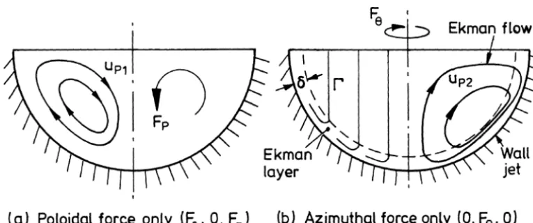
Ekman pumping is an inevitable by-product of swirl. Perhaps it is most simply understood in those special cases where the Lorentz force is purely azimuthal(Fp=0), and we briefly consider this case. In the absence of poloidal forcing, Ekman pumping takes the form of a wall jet as shown on the right of figure 3. That is to say, the swirl induces a secondary poloidal motion consisting of a high-speed wall jet (Ekman jet) which runs downward within the boundary layer (the Ekman layer) and recirculates back up through the (almost) inviscid core flow (Davidson [4]). The driving force for the wall jet is a radial pressure gradient which is established in the core of the flow in order to counterbalance the centripetal acceleration of the swirling fluid. In summary then, a steady flow is established in which each streamline spirals upward through the (almost) inviscid core and then back down through the Ekman layer.
Now this Ekman pumping is not an incidental feature of the flow, but rather controls the magnitude of the swirl (Davidson [4]). That is, in the steady state, the angular momentum and energy generated byFθ must be destroyed by shear stresses, and it is this balance between generation and dissipation which dictates the steady state value ofuθ. But the dissipation of energy is controlled by the Ekman pumping. It ensures that all the fluid particles are periodically flushed through thin, dissipative boundary layers, and this is the mechanism by which a steady flow is achieved. Note that, within the thin Ekman layersup∼uθ (Davidson [4]) and so by continuity the core recirculation is weak, of the order ofδuθ/R. (δis the boundary layer thickness.)
Figure 3. The left-hand figure shows the poloidal motion, up, driven directly by a poloidal force. The right-hand figure shows the angular momentum
Let us now return to the case in hand, where the dominant Lorentz force is poloidal. Suppose we have a pool of liquid metal into which we inject current (figure 1). The current may be injected at a single point on the axis, or else distributed across the top of the pool. It does not matter. The current density in the metal is poloidal and induces an azimuthal magnetic field, Bθ. Suppose that, in addition, we have a weak, “stray” magnetic field,Bz. Then F comprises a strong poloidal component, J×Bθ/ρ, plus a weaker azimuthal contribution, J×Bz/ρ. Now suppose that, at least initially, Bz is so small that the induced swirl is much weaker than the primary poloidal motion. The distribution of up is then uniquely determined by the poloidal force. Now consider the swirl. The governing equation for angular momentum,Ŵ=ruθ, is
DŴ
Here the subscript on νt indicates that we have in mind a turbulent flow which, for the present purpose, we model rather crudely using a turbulent eddy viscosity. Let the pool be a hemisphere of radiusR (the precise shape is not too important), and define an effective Reynolds number by Ret= |up|maxR/νt. When Ret is large (typically it has a value of∼100—see Section 5) the shear stresses are dominant only in the boundary layers. Outside these regions (4) simplifies to
Evidently, the angular momentum in each fluid particle rises as a result of the secondary azimuthal force and, provided boundary layers are avoided, this growth inŴis constrained only by the relatively weak shear stresses in the core. Consequently, large values of swirl can build up, even thoughFθis small. From (4), we can estimate uθ by equating the two terms on the right,
uθ/up∼ FθR/u2p
Ret.
Now suppose that we increaseFθ, with Fpfixed, up to the point whereuθand upare of similar magnitudes. (In practice we could do this by increasing the stray fieldBz.) We shall see that, for smalluθ, up scales roughly as u2
p/R∼Fp(inertia balances Lorentz force), and souθ∼upwhenFθ∼Re−t1|Fp| ∼0.01|Fp|. Thus a small but finite azimuthal force can give rise to an order one swirling motion. Onceuθ reaches a value of∼up,Ŵceases to play a passive role. It can react back on the poloidal motion through the centrifugal force(−u2
θ/r)erˆ . There now exists an intriguing possibility. Suppose thatŴis distributed in such a way that(−u2θ/r)erˆ balances Fp to within the gradient of a scalar:
−u2θ/rerˆ =Fp+ ∇φ+O Re−t 1. (6)
The driving force for poloidal motion disappears (φis absorbed in the pressure) and we are left with a swirling motion plus its associated (weak) Ekman pumping. If this were to occur then the energy of the poloidal flow should collapse asFθ approaches a value of∼0.01|Fp|. We shall see that is precisely what happens, and it is this which we refer to as poloidal suppression.
It seems counter intuitive that, as the level of (azimuthal) forcing increases, the energy of the flow should fall, and so we shall consider this idea in a little more detail. Suppose that we have increased Fθ (orBz) to a point where uθ ∼up. We have two obvious sources of poloidal motion, Fp and Ekman pumping. Let up1
be the poloidal flow driven directly by Fp (in the absence of swirl) and up2be the Ekman flow driven by the
directed. However, there is no real competition between up1 and up2 since the Ekman pumping is confined
to thin boundary layers and is very weak in the core. If these were the only two sources of poloidal motion, then asFθ increased up to a value of ∼0.01|Fp|we would expect to see no significant change in the energy of the poloidal motion. But there is a third source of poloidal motion. So far we have said nothing about the distribution ofŴ. We only know that, in the absence of a poloidal force,Ŵis independent ofzto leading order inνt (Davidson [4]). (This is true for any distribution of Fθ and represents a form of the Taylor–Proudman theorem.) However, if Ŵ varies withz then the resulting axial variation in the centrifugal force can drive a poloidal flow. NowŴis controlled by (4) which, outside the boundary layers, reduces to (5). Suppose that we can find distributions of upandŴwhich simultaneously satisfy the core equations (5) and (6) in the form:
up· ∇Ŵ=rFθ +O(νt), (7)
Then the poloidal force is effectively eliminated and the poloidal motion reduces to the weak Ekman pumping, up2. This not only dramatically reduces the energy of the poloidal flow, but also helps keepuθ at a modest level. That is, if the only poloidal motion is Ekman pumping, all of the streamlines will be flushed through the dissipative Ekman layers where the angular momentum created byFθ can be efficiently destroyed (see Section 3).
Evidently, if we can find core solutions for up and Ŵ which satisfy (7) and (8), then this represents an energetically favourable state. We shall see that these core equations are readily satisfied, for almost any distributions of current, and that the flow does indeed adopt this low energy state. The net result is that, when Fθ exceeds the modest threshold of ∼0.01|Fp|, the flow is dominated by swirl, despite the weakness of the azimuthal force. We believe that this is the phenomenon which is observed in laboratory experiments and industrial processes.
We shall spend the rest of this paper justifying this picture. In Section 2 we define our problem and state the governing equations. In Sections 3 and 4 we give analytical arguments in support of (7) and (8), and in Section 5 these are compared with numerical experiments. We conclude in Section 6. The primary novelty of our analysis lies in identifying: (a) Ekman pumping as the key dissipative mechanism; and (b) the almost complete elimination of the poloidal Lorentz force (and corresponding velocity) by the centrifugal force.
Most previous studies have focussed on the case where the current is introduced via a point electrode at r=0, z=0. (See, for example, Sozou and Pickering [6] or Bojarevics and Scherbinin [7].) In part, this is motivated by the existence of the self-similar solutions of the Navier–Stokes equation for a point source on the surface of a semi-infinite fluid. However, in our study we follow the example of Atthey [8] and consider the current to be introduced in a distributed fashion across the surface of the pool. There are several reasons for our choice. First, this characterizes most industrial processes, such as vacuum-arc remelting. Second, we wish to emphasize that the phenomenon is not related to the breakdown of the Jeffery–Hamel-like similarity solutions.
2. Governing equations and simplifying assumptions
and spreads radially outward as it passes down through the pool. It has poloidal components,(Jr,0, Jz), with Jr >0,Jz>0. (We use cylindrical polar coordinates(r, θ, z).) Faraday’s law reduces to the statement that J is irrotational while Ampere’s law relates J to its self field,Bθ:
Ampere: µJ= ∇ ×Bθeθˆ
In addition to the self field, we shall allow for a weak external magnetic field. For simplicity, we take this to be uniform and vertical. The Lorentz force (per unit mass) then has components
Fp= − Bθ2/ρµrˆer− ∇(pm/ρ), and (11)
Fθ=(Bz/ρµ) ∂Bθ
∂z , Bz=constant, (12)
wherepmis the magnetic pressureBθ2/2µ. Of course, we may absorbpminto the fluid pressure so that, without any loss of generality, we may drop the last term in (11). It is convenient to introduce the scaled magnetic field C=B/(ρµ)1/2, which has the dimensions of velocity. Our force components now become
Fp= −C
We shall take the flow to be turbulent and model the Reynolds stresses using a turbulent eddy viscosity,νt. In our numerical experiments the spatial distribution ofνt will be estimated using the populark–ε turbulence model. In this section and the next, however, we shall takeνt to be spatially uniform; in effect, we consider the laminar case. This is a gross simplification, but we are primarily interested in the structure and scaling of the flow and so it seems an appropriate starting point. (We shall see that Reynolds numbers based onνt, rather than ν, are of the order of 100.)
We shall assume axial symmetry. In such cases the poloidal velocity field, up, is uniquely determined by its vorticity,ωθ, while the distribution of swirl may be described in terms of angular momentum,Ŵ. The vorticity is related to the Stokes stream function,ψ, by
∇∗2ψ= ∇ ·r2∇ ψ/r2= −rωθ, up= ∇ ×
(ψ/r)eθˆ .
From (13), (14) and the Navier–Stokes equation, it is easy to show that the governing equations forωθ andŴ are
In terms of velocity, Eq. (16) may be uncurled to give the poloidal equation of motion:
Expressions (15)–(17) represent the final form of our governing equations of motion. However, it is convenience to introduce one last piece of notation:
b
Fp= u2θ−Cθ2/rerˆ . (18)
Evidently, Fpb represents the net driving force for poloidal motion. From (16) we see that, whenever Fpb is independent ofz, the poloidal motion vanishes.
Our final equation comes from (15). Integrating this over the domain yields the global torque balance introduced in Section 1:
We now consider solutions of these equations for small values ofFθ/|Fp|, but for moderate to high effective Reynolds numbers,upR/νt. We are particularly interested in solutions in whichuθ is dominant.
3. The role of Ekman pumping
In this section we shall show that our governing equations do indeed support solutions in which up≪uθ, despite the dominance of the poloidal forcing. As noted in Section 1, these solutions are based on the elimination of Fpby the centripetal acceleration, so thatFb=0 and the only poloidal motion is Ekman pumping. Outside the boundary layer, these solutions are characterized by (7) and (8) in the form
u· ∇Ŵ=rFθ, (20)
We claim that this is precisely the flow structure seen in the experiments of Bojarevics et al. [1].
In this section we shall verify the existence of solutions of the form (20)–(22). In Section 4 we argue that the solutions, while not unique, are the most likely to be seen in practice (providedFθ is not too small). Finally, in Section 5, we describe numerical experiments which support our assertions.
We are interested in flows in which Fθ ≪ |Fp| (i.e. Bz≪Bθ). First, however, it is convenient to briefly consider the reverse case, in whichBz≫Bθ, i.e. flows with strong azimuthal forcing but with a negligible poloidal force. This provides a convenient framework for reviewing the properties of Ekman dominated flows, which is an essential prerequisite for our discussion of poloidal suppression. We start then with flows in which Fθ≫ |Fp|, and then move to ones in which|Fp| ≫Fθ.
3.1. A review of Ekman pumping in flows with strong azimuthal forcing
Perhaps it is worth starting with a very simple example to establish the basic principles. Ekman pumping is very familiar in the context of spin-down of a fluid in an open-topped, cylindrical vessel. In such cases the fluid is set into a state of (almost) inviscid rotation by mechanical stirring. When the stirring is removed the fluid slows down by Ekman induced drag. Within the core of the flow the centrifugal force is balanced by a radial pressure gradient and this pressure gradient is imposed throughout the boundary layer on the base of the vessel. However, the swirl in this boundary layer is diminished through viscous drag and there is a corresponding reduction inu2
acceleration, causing a radial inflow at the base of the vessel. The fluid flows towards the axis, eventually drifting up and out of the boundary layer. Continuity then requires that the boundary layer is repleniched via the side walls, so a complete recirculation is established. As each fluid particle passes through the boundary layer it gives up a significant fraction of its kinetic energy and the fluid comes to rest when all of the contents of the vessel have been flushed through the Ekman layer.
Although this is a transient phenomenon, a similar process occurs in a steady flow subject to azimuthal forcing, F=Fθeθˆ (Davidson [4]). The first thing to note is that, for Ekman pumping to occur, it is unnecessary for the boundary and the axis of rotation to be mutually perpendicular. As indicated in figure 3(b), Ekman layers form whenever there is some component of rotation perpendicular to the surface. The second important point is that Ekman pumping is not an incidental feature of these forced flows, but rather it is an essential prerequisite for establishing a steady state. That is, if the Navier–Stokes equation is integrated around a closed streamline, we have
I
F·dℓ+νt
I
∇2u·dℓ=0, (23)
so that all of the energy imparted to the fluid by the Lorentz force F must be lost by viscous dissipation in the boundary layers. By implication, all streamlines must pass through a boundary layer and Ekman pumping provides the key entrainment mechanism. The structure of the flow is as shown in figure 3(b). It consists of an interior body of (almost) inviscid swirl, with high-speed wall jets on the inclined surfaces.
Within the Ekman layersuθ∼up and so, by continuity, the core recirculation is of orderuθδ/R. Now when Fp≪Fθ the core vorticity equation simplifies to
u· ∇(ωθ/r)=
(The subscriptc denotes values ofŴin the core of the flow.) Thus the contours of constant Ŵare vertical, as shown in figure 3(b). It is remarkable that the swirl is independent ofzno matter what the distribution ofFθ. This is a variant of the Taylor–Proudman theorem. The magnitude ofŴmay be estimated from the global torque balance (19). This givesŴ∼δ2Fθ/νt. A further estimate of the boundary layer thickness and eddy viscosity yieldsŴmax∼3F
We now return to the main concern of this paper: the case whereFθ is small and Fpis large.
3.2. Ekman pumping in flows with strong poloidal forcing(Fp≫Fθ)
Ekman layer (at the same radius). Now suppose we requireŴcto satisfy
Ŵc2=r2Cθ2+f (r), (24)
wheref (r)is an arbitrary function of radius. Then from (16) there is no source of poloidal motion, other than Ekman pumping. This guarantees entrainment of all of the streamlines and so provide an effective dissipation mechanism for the flow. We now explore the consequences of this distribution of swirl. We shall show that there is no contradiction between (24) and the azimuthal equation of motion.
If (24) is satisfied then the poloidal equations of motion (16) and (17) tells us nothing more about the core flow, other than the fact that Ekman pumping will occur. It remains to see if our assumed distribution ofŴ, (24), is consistent with the azimuthal equation of motion in the core, (15). Now suppose thatCz= −C0, where
C0>0. Since Bθ is a decreasing function of z this ensures that Ŵ >0. (Choosing Ŵ to be positive is an arbitrary but convenient choice. The arguments which follow work equally well ifŴis negative.) Equation (15) now becomes, in the core of the flow
u· ∇Ŵc= −rC0
Clearly, as each fluid particle spirals upward through the core its angular momentum increases. We now ask if this is consistent with our assumed distribution ofŴ: that is, are∂Ŵc/∂z <0,∂Ŵc/∂r >0 compatible with (24)? First we note that (24) gives
But this is exactly what is required. Second we rewrite (24) in the form
Ŵc2=Ŵcs2(r)+r2 Cθ2−Cθ s2(r). (26)
Now we are free to choose the distribution ofŴ2
cs(r)and so we can always arrange thatŴc increases withr. Once again, this is exactly what is required. It would seem, therefore, that our proposed distribution of swirl, (24), is compatible with the core azimuthal equation.
Finally, we must check that (24) is consistent with the azimuthal equation of motion in the Ekman layer. To this end we use (19), which may be rewritten as,
Z
rFθdV =π
I
cfŴcs2 ds. (27)
Typically,cf is of the order of 10−2 in a confined turbulent flow. (The precise value depends on Re.) Now the left-hand side of (27) is of orderC0CθR3while the right-hand side is at least of ordercfCθ2R
3. Thus, (27)
requiresC0>cfCθ, or equivalently,
Fθ >cf|Fp| ∼0.01|Fp|. (28)
It appears, therefore, that an Ekman dominated flow is physically realizable provided that Fθ is not too small. We shall see, in our numerical experiments, that this is exactly what happens. WhenFθ/|Fp|<10−3, uθ≪ |up|. In the range 10−3< Fθ/|Fp|<10−2the swirluθ grows to be of order|up|, and forFθ/|Fp|>10−2 we get Ekman pumping, with uθ ≫ |up|. It is remarkable that the velocity field should be dominated byuθ despite the relative weakness of the azimuthal forcing.
Finally, we note that, in the arguments above, we have made no assumption about the direction of the poloidal flow (whenFθ =0). Our arguments make no distinction between a flow which converges at the surface and one which diverges. We shall see that this is consistent with our numerical experiments.
4. Other possible flow structures
So far we have merely shown that our Ekman dominated flow, with Fp nullified by u2θ/r, represents one possible solution of the equations of motion (providedFθ is not too small). However, there are, in principle, other structures and scalings for u, and it is important that we identify these. For example, instead of destroying the angular momentum in the boundary layers we could let the swirl build up to a level at which distributed internal dissipation combats the generation of angular momentum. Indeed, this must represent the flow structure forFθ <∼0.01|Fp|where there is no Ekman pumping. To see how such a flow might come about consider (15) and (19) written in the form
where (30) now applies to any volume bounded by a streamline closed int ther–z plane. We now look for a solution without Ekman pumping, in which the bulk of the streamlines avoid the boundary layers. From (30) the forcing and diffusive terms must be of similar magnitudes and so, for high Ret, (29) demands that u· ∇Ŵis of orderνt. It follows that
Ŵ=Ŵ(ψ)+O(νt).
Note thatŴis almost constant along the streamlines. Now (30) says that a steady state is achieved when all of the angular momentum created byrFθ diffuses across the streamlines to the boundary. Consequently, the level ofŴ will rise in the core of the flow until the right-hand integral in (30) balances the generation term on the left. All of this happens subject to the boundary conditionŴ=0 at the outer surface.
This situation is analogous to injecting heat into a prescribed recirculating flow and letting the internal temperature rise until such time as the diffusion of heat out to the boundary balances the internal generation of heat. Now if the outer boundary condition is one of constant temperature, we would not expect a thermal boundary layer to develop. Rather, we will have relatively uniform cross-stream gradients in temperature throughout the flow. We would expect the same to be true for angular momentum. That is, there will be a smooth decline inŴfrom its elevated value at the centre of the flow to zero at the boundary. Indeed, we may estimate the cross-stream gradients inŴfrom (30). If Re is large enough then Ŵ≈Ŵ(ψ)and (30) yields the estimate
It seems plausible, therefore, that there are at least two structures forŴ. In the Ekman dominated flowŴis distributed in such a way thatu2θ/r eliminates the poloidal forcing. All streamlines are then flushed through the boundary layers by Ekman pumping. The level of swirl is fixed by the balance between the distributed generation of angular momentum and dissipation ofŴ in the Ekman layers. In the second option there is no such balance betweenu2
θ and Fp. Rather, the poloidal flow is dictated, at least in part, by the poloidal forcing and there is no reason to suppose that the streamlines are entrained in the boundary layers. In such a case a high value of Ret requiresŴ=Ŵ(ψ)+O(νt). The swirl builds up until such time as the cross-stream diffusion of angular momentum balances the generation ofŴby the azimuthal force. The essential difference between the two structures is the manner in whichŴis transported to the boundaries. In one case it is advected to the boundaries, in the other it diffuses.
We shall see in the next section that, providedFθ >∼0.01|Fp|, the Ekman dominated structure is preferred. Perhaps this is not surprising. The global integral (30) givesŴ∼δ2F
θνt for the Ekman flow butŴ∼R2Fθ/νt for the diffusive case. (For the Ekman case,Ŵ∼Fθ5/9. See Section 3.2.) The Ekman structure leads to a lower kinetic energy, both for the swirling and the poloidal components of the flow. However, for values ofFθ less than∼0.01|Fp|, the azimuthal torque is not sufficiently large to maintain Ekman pumping and so we might expect the diffusive structure to be seen.
5. Numerical experiments
We have calculated the flow of liquid steel (ν=7.8×10⁻⁷m2/s) in a hemispherical pool of radiusR=0.1 m.
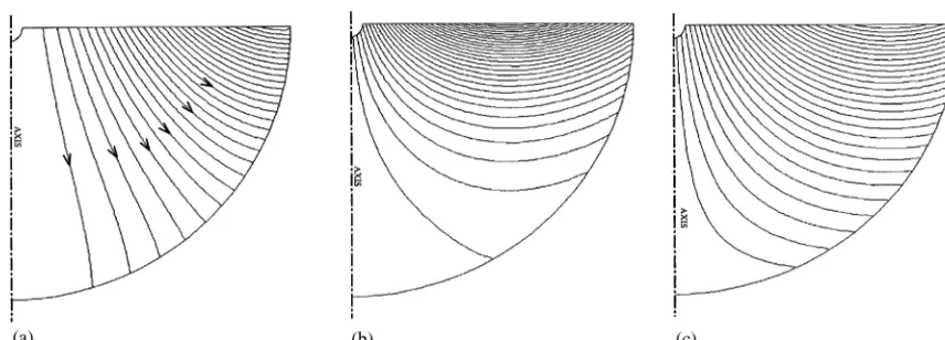
The current is taken to be uniform over the top surface of the pool. Its distribution is controlled by the boundary condition we set for J. We have specified that the current leaves the cylindrical volumer =R,z=R at right angles to that surface. (This is an arbitrary but convenient choice.) The resulting distribution of J is shown in
figure 4(a). The current passes down through the pool and the surrounding solid metal, spreading radially as it
does so. The corresponding distribution for the self field,Bθ, is
Cθ=CJb 1(δ1r/R)cosh δ1(1−z/R)
J1(δ1)cosh(δ1)
, (32)
whereδ1is the first zero of the Bessel functionJ0. The parameterCbrepresents the peak value ofCθ, which we have taken as 1 m/s. (This corresponds to a peak field of around 0.1 Tesla.) We have also allowed for an axial
Figure 4. Current and magnetic forces in the liquid metal pool. (a) Current flow. (b) Contours of constant values ofFr(30 equally spaced contours).
magnetic fieldCz= −C0, whereC0lies in the range 0–1 m/s. (The choice of a negative value forCzensures thatŴ >0.) The Lorentz force per units mass is calculated from (13) and (14):
F= −C2θ/r,−C0∂Cθ/∂z,0
. (33)
The contours of constantFr and Fθ (for C0=0.01) are shown in figures 4(b) and 4(c) respectively. We may
takeC0/Cb as a measure of relative size ofFθ/|Fp|.
The flow is taken to be turbulent (Re∼105) and we have estimated the Reynolds stresses τ
ij using the populark–εone-point closure model. Like all closure schemes this is flawed and is unlikely to give particularly accurate estimates ofτij, although it should provide estimates which are at least qualitatively correct. This is adequate for the present purpose since we are interested primarily in the general structure and scaling of these flows. (Thek–εscheme is an eddy viscosity model in whichνt is taken to scale asνt∼ℓmk1/2, wherekis the turbulent kinetic energy and the mixing length,ℓm, is estimated from an empirical transport equation. See, for example, Rodi [9].)
The equations of motions were solved using standard finite-difference methods employing quadratic upwind differencing for the advection terms. The flow was taken as axisymmetric and a grid consisting of 48×51
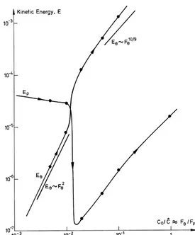
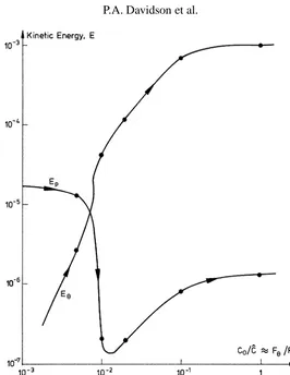
Figure 5. Variation of kinetic energy of the swirling(Eθ)and poloidal(Ep)components of motion as the ratioFθ/Fpis increased. (The poloidal flow
elements was used. Increasing the grid by a factor of four, to 87×100 elements, produced a change of 0.3–0.8% in the calculated value of|uθ|max. The resolution offered by a 48×51 grid seems, therefore, to be adequate.
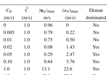
WithCb fixed at 1 m/s we have calculated the flow for a range of values ofC0, corresponding toC0/Cb=0,
0.005, 0.01, 0.02, 0.05, 0.1 and 1.0. This represents the full range fromFθ =0 toFθ ∼ |Fp|. The resulting variation of the kinetic energiesEθ and Ep (defined as the integrals ofu2θ/2 and u
2
p/2) are shown in figure 5. Note that when the azimuthal force reaches a values of∼0.01|Fp|, the swirl and poloidal motions have similar intensities. As Fθ is further increased, the energy of the poloidal motion collapses, dropping by a factor of 100. This is exactly the behaviour anticipated in Section 3. We shall see that, forFθ <∼0.01|Fp|, there is no Ekman pumping and the poloidal flow is dominated by Fp, the swirl being too weak to react back in up. For Fθ >∼0.01|Fp| the poloidal flow is virtually eliminated through the balance Fp∼ −(u2θ/r)erˆ + ∇φ. What little poloidal motion there is corresponds to Ekman pumping. Note also that, for low values ofFθ,uθ scales asuθ ∝Fθ, which is precisely the behaviour we would expect for the diffusive structure (31). For large Fθ, on the other hand, we haveuθ ∝Fθ5/9, which is what we would anticipate in an Ekman dominated flow (see Section 3). The effective Reynolds number Ret = |up|maxR/νt also changes as we move through the transition Fθ∼0.01|Fp|. For low values ofFθ we have Ret∼60 (based on a spatially averaged value ofνt), while high values ofFθ lead to Ret ∼400. To the extent that we have faith in the turbulence closure model, this indicates that there is a fall in the turbulence level once Ekman pumping sets in. This seems physically plausible.
The maximum values of|up|and uθ from the different cases are given in table I. Note that, whenFθ =0, we have|up| ∼Cb∼(FpR)1/2, as suggested in Section 1. This indicates that the scaling of the poloidal motion is dictated by inertia∼Lorentz force. (This scaling is well established for similar poloidal MHD flows such as those which occur in induction furnaces. See, for example, Moore and Hunt [10].)
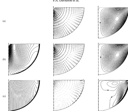
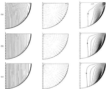
The flow patterns for the cases C0=0, 0.01 and 0.05 are shown in figure 6. The transition to an Ekman
dominated structure is quite striking. The flows for the cases C0=0.1 and 1.0 are shown in figure 7 and
compared with the case where the poloidal forcing is removed(C0=1.0, Cb=0). Again, the motion is clearly
dominated by Ekman pumping. It is remarkable that removing the poloidal forcing altogether makes almost no difference to the flow pattern. It is even more remarkable that, when the azimuthal forcing is only a few percent of the Fp, the motion is dominated by swirl.
Figure 6. Contours of constantuθ, poloidal velocity and poloidal streamfunction for (a)C0=0, (b)C0=0.01 and (c)C0=0.05.
absence of azimuthal forcing is shown in figure 8(b). It diverges from the axis at the surface. Figure 9 shows the variation ofEθ andEp asFθ/|Fp|is increased from zero. Qualitatively we have precisely the same behaviour as before. WhenFθ reaches a value of ∼0.01|Fp| then u2θ ∼u2p. At higher values of Fθ the energy of the poloidal motion collapses as Ekman dominated structure emerges. Evidently, the phenomenon is not restricted to a radially converging base flows.
6. Discussion
Our numerical experiments are broadly in line with the theoretical analysis of Section 2. It seems that the phenomenon of poloidal suppression is quite unrelated to the direction of the base flow (it may converge or diverge at the surface) and is not a manifestation of the breakdown of the Jeffrey–Hamel-like point-electrode flow. It results from a suppression of the poloidal motion through the balance u2θ/r ∼Fp. This allows the poloidal motion to be dominated by Ekman pumping which, in turn, ensures that every streamline is flushed through a thin, dissipative Ekman boundary layer. The result is a flow of low energy (Epis virtually eliminated while Eθ scales asF
10/9
Figure 7. Contours of constant uθ, poloidal velocity vectors and poloidal streamfunction for (a) C0=0.1, Cb=1.0, (b) C0=1.0, Cb=1.0, (c)C0=1.0,Cb=0.
(a) (b)
Figure 9. Variation of kinetic energy of the swirling(Eθ)and poloidal(Ep)motion asFθ/Fpis increased.
We also believe our theory is broadly in line with the experimental evidence. For example, the traditional explanation predicts the appearance of swirl of Re∼4–5, and attributes it to the breakdown of point electrode, self similar solution. However, in the experiments of Bojarevics we have Re=200–300, and in Vacuum-arc remelting furnaces, where this phenomenon is also seen, the current is uniformly distributed across the pool surface. This is more consistent with our explanation.
In the examples considered here the poloidal motion has been suppressed by the radial stratification of angular momentum. But there is a well known analogy between buoyancy-driven and swirling flows. It is intriguing to ask whether or not a similar phenomenon may occur when there is a competition between thermal forces, which tend to give rise to an axial stratification of density, and a poloidal MHD force. That is, when the thermal forces exceed some threshold, does the poloidal motion disappear, except in the thermal boundary layers? This is of considerable interest in certain metallurgical processes and is the subject of our current investigations. Preliminary results suggest that there is indeed a strong analogy. That is, the Ekman layers are replaced by thermal boundary layers and the core equations (20) and (21) are replaced by
u· ∇T =0, (34)
∂ ∂z
C2
θ r
=gβ∂T
∂r, (35)
References
[1] Bojarevics V., Millere R., Chaikovsky A.I., Investigation of the azimuthal perturbation growth in the flow due to an electric current point source, in: Proc. 10th Riga Conference on MHD, Vol. 1, Salaspils, 1981, pp. 147–148.
[2] Moreau R., Magnetohydrodynamics, Kluwer, Dordrecht, 1990.
[3] Davidson P.A., Short D.J., Kinnear D., The role of Ekman pumping in confined, electromagnetically-driven flow, Eur. J. Mech. B-Fluids 14 (6) (1995) 793–821.
[4] Davidson P.A., Swirling flow in an axisymmetric cavity driven by a rotating magnetic field, J. Fluid Mech. 245 (1992) 669–699. [5] Shtern V., Barrero A., Bifurcation of swirl in liquid cones, J. Fluid Mech. 300 (1995) 169–205.
[6] Sozou C., Pickering W.M., Magnetohydrodynamic flow due to the discharge of an electric current in a hemisphere, J. Fluid Mech. 73 (1976) 641–650.
[7] Bojarevics V., Scherbinin E.V., Azimuthal rotation in the axisymmetric meridional flow due to an electric current source, J. Fluid Mech. 126 (1983) 413–430.
[8] Atthey D.R., A mathematical model for fluid flow in a weldpool at high currents, J. Fluid Mech. 98 (1980) 878–801. [9] Rodi W., Turbulence models and their application in hydraulics—A state of the art review, IAHR, 1984.
![Figure 2. Geometry analysed by Shtern and Barrero [5]. Rather than consider a flat surface they investigated flows in a semi-infinite domain with aconical surface.](https://thumb-ap.123doks.com/thumbv2/123dok/3123105.1379721/4.595.130.425.76.260/figure-geometry-analysed-barrero-consider-investigated-innite-aconical.webp)