www.elsevier.com / locate / econbase
The robustness of tests for seasonal differencing to structural
breaks
*
Artur C.B. da Silva Lopes
˜
Instituto Superior de Economia e Gestao (ISEG–UTL), Rua do Quelhas 6, 1200 Lisboa, Portugal
Received 24 May 2000; received in revised form 4 December 2000; accepted 21 December 2000
Abstract
Monte Carlo simulations are used to compare the power properties of three simple tests for the seasonal differencing filter when the data contain seasonal mean shifts. Overall, the results favour the HEGY–GLN test.
2001 Elsevier Science B.V. All rights reserved.
Keywords: Seasonal integration; Tests; Structural breaks; Monte Carlo
JEL classification: C22; C52
1. Introduction
Simple tests for determining the order of seasonal integration are becoming increasingly popular for seasonally unadjusted quarterly data. Given the possible pitfalls associated with the use of the deterministic seasonal stationary model (see Franses et al., 1995; Lopes, 1999) and the traditional practice in time series analysis, such tests are useful to assess the adequacy of the seasonal (or annual) differencing filter. This, in turn, is often considered as a simple and useful filter to adjust for seasonality and to remove stochastic non-stationarity (both seasonal and non-seasonal). Nevertheless, the issue of comparing the power properties of some simple tests designed for that purpose has been rarely addressed. Two important exceptions are the papers by Ghysels (1994), henceforth GLN, and
1
by Hylleberg (1995) .
On the other hand, since the seminal paper by Perron (1989), economists are aware that the procedures used for testing stochastic non-stationarity may suffer from severe power problems when structural breaks are present in a (segmented trend) stationary data generation process but are
*Corresponding author. Tel.: 1351-21-3922-796; fax: 1351-21-392-2781. E-mail address: [email protected] (A.C.B. da Silva Lopes).
1
In Rodrigues and Osborn (1999) this issue is investigated for monthly data.
neglected in the testing strategy. A similar problem may afflict tests for seasonal integration, i.e., one may conjecture that spurious evidence for seasonal differencing may emerge frequently when there is
2
a structural break in a process containing only deterministic seasonality .
The purpose of this paper is to compare, through Monte Carlo methods, the power properties of three simple tests for the seasonal differencing filter when the data contain (deterministic) seasonal mean shifts. These are the Dickey et al. (1984) (DHF), the Osborn et al. (1988) (OCSB), and the Hylleberg et al. (1990) (HEGY) tests. In the next section a brief review of these tests is presented. Section 3 contains the simulation results and Section 4 draws the most important conclusions for empirical work. The critical values used for the simulations are presented in Appendix A.
2. Simple tests for the seasonal differencing filter
For quarterly data, the seasonal differencing filter can be written as
4
where L denotes the usual lag operator and i 5 21. The DHF test for this filter is a straightforward
extension of the Dickey–Fuller test to the case of seasonal (quarterly) data. It is based on the regression
p
D4yt5mt1a yt241
O
g Di 4yt2i1et, (2)i51
where y (tt 51, 2, . . . , T ) often represents some log transformed series, m denotes the appropriatet
2
deterministic component, p is the order of lag augmentation and et|iid(0, se). The most popular
version of the test is based on the simple t-ratio for testing H :0a50 against H :1a,0. As pointed out
by GLN and by Rodrigues and Osborn (1999), its main drawback is that it is designed against stationary seasonal alternatives only.
4
The OCSB test was originally proposed as a test for theDD45(12L )(12L ) filter (i.e., for the
I(1, 1) hypothesis, according to the OCSB definition). Only recently the simpler version for the D4 filter was put forward by Rodrigues and Osborn (1999). This version is based on the regression
p
D4yt5mt1b1S(L )yt211b2 yt241
O
f Di 4yt2i1et, (3)i51
3
and the test statistic is given by the F-statistic for testing H :0b15b250 .
In contrast to the previous tests, the HEGY statistics allow testing separately the different
2
Following conjectures in Ghysels (1994) and in Franses and Vogelsang (1998), this issue was recently investigated by ˜ ´
Smith and Otero (1997) and by Lopes and Montanes (1999) in what concerns only the popular tests of Hylleberg et al. (1990).
3
nonseasonal (1) and seasonal (21, 1i and 2i ) unit roots implied by theD4 filter (see Eq. (1)). The HEGY regression is based precisely on the previous root factorization and it is given by
p
D4yt5mt1p1 y1,t211p2 y2,t211p3y3,t221p4 y3,t211
O
u Di 4yt2i1et, (4)i51
2 2
where y1t5S(L )y , yt 2t5 2(12L )(11L )y and yt 3t5 2(12L )y . Ghysels et al. (1994) (GLN)t
extended the HEGY procedure for testing the adequacy of the D4 filter, proposing the F-statistic for
H :0 p15p25p35p450 (F1234). Thus, this test will be called HEGY–GLN.
A seemingly different test statistic was recently proposed by Kunst (1997). This is given by the
F-statistic for H :0 a15a25a35a450 in the regression equation
p
D4yt5mt1a1 yt211a2yt221a3 yt231a4 yt241
O
u Di 4yt2i1et. (5)i51
However, as noticed by Osborn and Rodrigues (1999), it coincides with the HEGY–GLN statistic because the regressors in (4) are simple linear transformations of those in (5). Given the well known invariance of OLS estimators and residual-based test statistics to (non-singular) linear transformations of linear models, the numerical identity is clear. Additionally, it should be also clear that the OCSB test may lack power relatively to the Kunst (HEGY–GLN) test, as Eq. (3) can be written as
p
D4yt5mt1b1( yt211yt221yt23)1(b11b2) yt241
O
f Di 4yt2i1et, (6)i51
which shows that the restrictionsa15a25a3 are imposed on Eq. (5). The restrictions implicit in the
DHF test are also clear: a15a25a350.
3. Monte Carlo experiments: design and results
Given the almost universal consensus about the presence of a nonseasonal unit root in economic time series, the data generation process (DGP) is given by
4 4
Dyt5
O
giDit1O
diD [Iit t.t]1´t, (7)i51 i51
where D (iit 51, 2, 3, 4) represent the usual seasonal dummy variables, [It.t] is 1 when t.t and zero
otherwise, t denotes the time of the break (andt5lT, 0,l,1, l representing the fraction break
parameter), and´t|nid(0, 1). Hence, there is at most one shift in each season, the pre- and post-break
seasonal cycles being given by thegi and thegi1di magnitudes respectively. Thus, thedi parameters
represent the seasonal mean shifts. Furthermore, to mimic the behavior of trending data, 2g15g25
4 4
2g351 andg452, so that before the break the annual drift isoi51 ig51 . As the structural break is
4
neglected, in all the test regressions mt5oi51ciDit1bt. Moreover, since this analysis is concerned
only with power problems, p was always set to zero.
4
As usual, the power estimates are based on 5% significance level tests (whose critical values are
presented in Appendix A) and are computed using 10 000 replications. Sample sizes with T548, 96
and 160 were considered and the symbol ‘¯1.0’ denotes an estimate lying in the interval [0.9995,
0.9999].
For comparison purposes, Table 1 presents the power estimates for the no-break case (d15d25
d35d450). As besides the deterministic and the stochastic trends the data contain only deterministic
seasonality, the excellent performance of the OCSB and HEGY-GLN tests is not surprising. Given the results reported in GLN, the poor behavior of the DHF test was also expected. However, this could legitimate excluding it from further consideration.
To simplify the analysis, a single break parameter, d(51, 3, 5), is used. However, this will be
enough to generate several interesting situations:
5
Case 1: change in the annual drift only, d15d25d35d45d ;
Case2: change in both the annual drift and the seasonal pattern, the break affecting only one of the
seasons, e.g., d15d,d25d35d450.
4
For the other cases only the seasonal cycle changes, i.e., oi51 id 50:
Case3: only two contiguous quarters are affected symmetrically, as whend15 2d25d,d35d45
0;
Case 4: only two non-contiguous quarters are affected symmetrically, e.g., d15 2d35d, d25
d450;
Case 5:d15d35 2d25 2d45d and
Case 6:d15d25 2d35 2d45d, i.e., all the seasons are affected, the difference between these
two cases lying again on the disturbed periodicities.
Table 2 presents the power estimates whenl50.5, i.e., when the break occurs in the middle of the
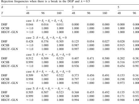
sample. The main conclusions that can be drawn from it are the following:
(a) As expected, and particularly when the break magnitude is large and the sample size is small, the presence of seasonal mean shifts affects the power performance of all the tests.
(b) However, in spite of the break, both the OCSB and the HEGY–GLN tests seem to remain
consistent, and even for breaks as large as d55 (553s´) the power recovery is almost always
completed when T5160. The only exception is observed for the OCSB test in case 6.
Table 1
Rejection frequencies when there is no break in the DGP
T 48 96 160
DHF 0.524 0.527 0.519
OCSB ¯1.0 1.000 1.000
HEGY 1.000 1.000 1.000
5
Table 2
Rejection frequencies when there is a break in the DGP andl 50.5
d 1 3 5
T 48 96 160 48 96 160 48 96 160
case 1:d 5 d 5 d 5 d 5 d1 2 3 4
DHF 0.044 0.016 0.011 0.000 0.000 0.000 0.000 0.000 0.000
OCSB ¯1.0 1.000 1.000 1.000 1.000 1.000 1.000 1.000 1.000
HEGY–GLN ¯1.0 1.000 1.000 1.000 1.000 1.000 1.000 1.000 1.000
case 2:d 5 d1,d 5 d 5 d 52 3 4 0
DHF 0.428 0.376 0.305 0.125 0.054 0.027 0.028 0.010 0.007
OCSB ¯1.0 1.000 1.000 0.987 1.000 1.000 0.915 1.000 1.000
HEGY–GLN ¯1.0 1.000 1.000 0.997 1.000 1.000 0.976 1.000 1.000
case 3:d 5 d 5 2 d1 2,d 5 d 53 4 0
DHF 0.512 0.509 0.525 0.407 0.471 0.500 0.202 0.383 0.455
OCSB 0.999 1.000 1.000 0.889 1.000 1.000 0.316 0.979 1.000
HEGY–GLN ¯1.0 1.000 1.000 0.936 1.000 1.000 0.454 0.993 1.000
case 4:d 5 d 5 2 d1 3,d 5 d 52 4 0
DHF 0.509 0.507 0.522 0.373 0.456 0.491 0.153 0.341 0.433
OCSB 0.998 1.000 1.000 0.797 ¯1.0 1.000 0.198 0.920 ¯1.0
HEGY–GLN ¯1.0 1.000 1.000 0.992 1.000 1.000 0.973 1.000 1.000
case 5:d 5 d 5 d 5 2 d 5 2 d1 3 2 4
DHF 0.505 0.507 0.523 0.368 0.455 0.492 0.135 0.335 0.434
OCSB 0.999 1.000 1.000 0.809 1.000 1.000 0.171 0.932 1.000
HEGY–GLN ¯1.0 1.000 1.000 0.994 1.000 1.000 0.988 1.000 1.000
case 6:d 5 d 5 d 5 2 d 5 2 d1 2 3 4
DHF 0.489 0.502 0.521 0.242 0.396 0.463 0.048 0.204 0.343
OCSB 0.993 1.000 1.000 0.453 0.989 1.000 0.033 0.457 0.974
HEGY–GLN 0.999 1.000 1.000 0.993 1.000 1.000 0.997 1.000 1.000
(c) On the contrary, for cases 1 and 2, the DHF test seems to exhibit an extreme form of inconsistency, the power approaching zero as T grows. Clearly, this is an additional argument against the use of this test. Notice also that the DHF test is always clearly dominated by the other two.
(d) Even for a moderately large break (d53) and for relatively small samples (T596), the power
of the OCSB and HEGY–GLN tests is unaffected in almost every case. The only exception occurs with the OCSB test in case 6 but the power loss barely exceeds 1%.
(e) However, particularly for small samples (T548 and 96), the HEGY–GLN test should be
preferred to the OCSB test because its power loss can be much smaller when the break is moderate or large. In other words, the HEGY–GLN test is more robust to the size of the break, its power functions dominating those of the OCSB test.
Finally, unreported results (available from the author upon request) show that for almost every case, and even when T is as small as 96, the power functions for the OCSB and the HEGY–GLN tests are
Table A.1
5% critical values for the seasonal differencing tests
T 48 96 160 400
DHF 24.43 24.36 24.32 24.31
OCSB 11.48 11.03 10.87 10.69
HEGY–GLN 6.72 6.47 6.34 6.20
4. Concluding remarks
For most empirical situations, i.e., for samples covering at least 24 years of quarterly observations
(T$96) and for small and moderately large breaks (d#3), the HEGY–GLN test maintains its power
properties intact and the behavior of the OCSB test is very close to this. However, in small samples the power performance of the HEGY–GLN is the most robust to large breaks. Thus, preference should be given to this test. The results also clearly suggest avoiding the use of the DHF test.
Acknowledgements
I am grateful to an anonymous referee and to J. Santos Silva and Uwe Hassler for useful
˜ ˆ
suggestions. The usual disclaimer applies. Financial support from Fundac¸ao para a Ciencia e Tecnologia through Programa POCTI is also gratefully acknowledged.
Appendix A
Table A.1 presents the 5% critical values used for the Monte Carlo simulations, the auxiliary test
4
regressions being (2), (3) and (4), with mt5oi51ciDit1bt (and P50), using a DGP given by
D4yt5et, et|nid(0,1), and based on 40 000 replications.
References
Dickey, D.A., Hasza, D.P., Fuller, W.A., 1984. Testing for unit roots in seasonal time series. Journal of the American Statistical Association 79, 355–367.
Franses, P.H., Hylleberg, S., Lee, H.S., 1995. Spurious deterministic seasonality. Economics Letters 48, 249–256. Franses, P.H., Vogelsang, T., 1998. On seasonal cycles, unit roots, and mean shifts. The Review of Economics and Statistics
80, 231–240.
Ghysels, E., 1994. On the economics and econometrics of seasonality. In: Sims, C.A. (Ed.). Advances in Econometrics, Sixth World Congress, Vol. I. Cambridge University Press, pp. 257–322.
Ghysels, E., Lee, H.S., Noh, J., 1994. Testing for unit roots in seasonal time series. Journal of Econometrics 62, 415–442. Hylleberg, S., 1995. Tests for unit roots: general to specific or specific to general? Journal of Econometrics 69, 5–25. Hylleberg, S., Engle, R.F., Granger, C.W.J., Yoo, B.S., 1990. Seasonal integration and cointegration. Journal of Econometrics
49, 215–238.
Lopes, A.C.B. da S., 1999. Spurious deterministic seasonality and autocorrelation corrections with quarterly data: further Monte Carlo results. Empirical Economics 24, 341–359.
˜ ´
Lopes, A.C.B. da S., Montanes, A., 1999. The behaviour of seasonal unit root tests for quarterly time series with seasonal mean shifts. CEMAPRE Working Paper 99-10 (revised version in 2000).
Osborn, D.R., Chui, A.P.L., Smith, J.P., Birchenhall, C.R., 1988. Seasonality and the order of integration for consumption. Oxford Bulletin of Economics and Statistics 50, 361–377.
Osborn, D.R., Rodrigues, P.M.M., 1999. Asymptotic distributions of seasonal unit root tests: a unifying approach, mimeo. Perron, P., 1989. The great crash, the oil shock and the unit root hypothesis. Econometrica 57, 1361–1402.
Rodrigues, P.M.M., Osborn, D.R., 1999. Performance of seasonal unit root tests for monthly data. Journal of Applied Statistics 26, 985–1004.