Statistical Pattern Recognition
Statistical Pattern Recognition
Second Edition
First edition published by Butterworth Heinemann.
Copyright c2002 John Wiley & Sons Ltd, The Atrium, Southern Gate, Chichester, West Sussex PO19 8SQ, England
Telephone (+44) 1243 779777
Email (for orders and customer service enquiries): [email protected] Visit our Home Page on www.wileyeurope.com or www.wiley.com
All Rights Reserved. No part of this publication may be reproduced, stored in a retrieval system or transmitted in any form or by any means, electronic, mechanical, photocopying, recording, scanning or otherwise, except under the terms of the Copyright, Designs and Patents Act 1988 or under the terms of a licence issued by the Copyright Licensing Agency Ltd, 90 Tottenham Court Road, London W1T 4LP, UK, without the permission in writing of the Publisher. Requests to the Publisher should be addressed to the Permissions Department, John Wiley & Sons Ltd, The Atrium, Southern Gate, Chichester, West Sussex PO19 8SQ, England, or emailed to [email protected], or faxed to (+44) 1243 770571.
This publication is designed to provide accurate and authoritative information in regard to the subject matter covered. It is sold on the understanding that the Publisher is not engaged in rendering professional services. If professional advice or other expert assistance is required, the services of a competent professional should be sought.
Other Wiley Editorial Offices
John Wiley & Sons Inc., 111 River Street, Hoboken, NJ 07030, USA
Jossey-Bass, 989 Market Street, San Francisco, CA 94103-1741, USA
Wiley-VCH Verlag GmbH, Boschstr. 12, D-69469 Weinheim, Germany
John Wiley & Sons Australia Ltd, 33 Park Road, Milton, Queensland 4064, Australia
John Wiley & Sons (Asia) Pte Ltd, 2 Clementi Loop #02-01, Jin Xing Distripark, Singapore 129809
John Wiley & Sons Canada Ltd, 22 Worcester Road, Etobicoke, Ontario, Canada M9W 1L1
British Library Cataloguing in Publication Data
A catalogue record for this book is available from the British Library
ISBN 0-470-84513-9(Cloth) ISBN 0-470-84514-7(Paper)
Typeset from LaTeX files produced by the author by Laserwords Private Limited, Chennai, India Printed and bound in Great Britain by Biddles Ltd, Guildford, Surrey
To Rosemary,
Contents
Preface xv
Notation xvii
1 Introduction to statistical pattern recognition 1
1.1 Statistical pattern recognition 1
1.1.1 Introduction 1
1.1.2 The basic model 2
1.2 Stages in a pattern recognition problem 3
1.3 Issues 4
1.4 Supervised versus unsupervised 5
1.5 Approaches to statistical pattern recognition 6
1.5.1 Elementary decision theory 6
1.5.2 Discriminant functions 19
1.6 Multiple regression 25
1.7 Outline of book 27
1.8 Notes and references 28
Exercises 30
2 Density estimation – parametric 33
2.1 Introduction 33
2.2 Normal-based models 34
2.2.1 Linear and quadratic discriminant functions 34
2.2.2 Regularised discriminant analysis 37
2.2.3 Example application study 38
2.2.4 Further developments 40
2.2.5 Summary 40
2.3 Normal mixture models 41
2.3.1 Maximum likelihood estimation via EM 41
2.3.2 Mixture models for discrimination 45
2.3.3 How many components? 46
2.3.4 Example application study 47
2.3.5 Further developments 49
viii CONTENTS
2.4 Bayesian estimates 50
2.4.1 Bayesian learning methods 50
2.4.2 Markov chain Monte Carlo 55
2.4.3 Bayesian approaches to discrimination 70
2.4.4 Example application study 72
2.4.5 Further developments 75
2.4.6 Summary 75
2.5 Application studies 75
2.6 Summary and discussion 77
2.7 Recommendations 77
2.8 Notes and references 77
Exercises 78
3 Density estimation – nonparametric 81
3.1 Introduction 81
3.2 Histogram method 82
3.2.1 Data-adaptive histograms 83
3.2.2 Independence assumption 84
3.2.3 Lancaster models 85
3.2.4 Maximum weight dependence trees 85
3.2.5 Bayesian networks 88
3.2.6 Example application study 91
3.2.7 Further developments 91
3.2.8 Summary 92
3.3 k-nearest-neighbour method 93
3.3.1 k-nearest-neighbour decision rule 93
3.3.2 Properties of the nearest-neighbour rule 95
3.3.3 Algorithms 95
3.3.4 Editing techniques 98
3.3.5 Choice of distance metric 101
3.3.6 Example application study 102
3.3.7 Further developments 103
3.3.8 Summary 104
3.4 Expansion by basis functions 105
3.5 Kernel methods 106
3.5.1 Choice of smoothing parameter 111
3.5.2 Choice of kernel 113
3.5.3 Example application study 114
3.5.4 Further developments 115
3.5.5 Summary 115
3.6 Application studies 116
3.7 Summary and discussion 119
3.8 Recommendations 120
3.9 Notes and references 120
CONTENTS ix
4 Linear discriminant analysis 123
4.1 Introduction 123
4.2 Two-class algorithms 124
4.2.1 General ideas 124
4.2.2 Perceptron criterion 124
4.2.3 Fisher’s criterion 128
4.2.4 Least mean squared error procedures 130
4.2.5 Support vector machines 134
4.2.6 Example application study 141
4.2.7 Further developments 142
4.2.8 Summary 142
4.3 Multiclass algorithms 144
4.3.1 General ideas 144
4.3.2 Error-correction procedure 145
4.3.3 Fisher’s criterion – linear discriminant analysis 145
4.3.4 Least mean squared error procedures 148
4.3.5 Optimal scaling 152
4.3.6 Regularisation 155
4.3.7 Multiclass support vector machines 155
4.3.8 Example application study 156
4.3.9 Further developments 156
4.3.10 Summary 158
4.4 Logistic discrimination 158
4.4.1 Two-group case 158
4.4.2 Maximum likelihood estimation 159
4.4.3 Multiclass logistic discrimination 161
4.4.4 Example application study 162
4.4.5 Further developments 163
4.4.6 Summary 163
4.5 Application studies 163
4.6 Summary and discussion 164
4.7 Recommendations 165
4.8 Notes and references 165
Exercises 165
5 Nonlinear discriminant analysis – kernel methods 169
5.1 Introduction 169
5.2 Optimisation criteria 171
5.2.1 Least squares error measure 171
5.2.2 Maximum likelihood 175
5.2.3 Entropy 176
5.3 Radial basis functions 177
5.3.1 Introduction 177
5.3.2 Motivation 178
x CONTENTS
5.3.4 Radial basis function properties 187
5.3.5 Simple radial basis function 187
5.3.6 Example application study 187
5.3.7 Further developments 189
5.3.8 Summary 189
5.4 Nonlinear support vector machines 190
5.4.1 Types of kernel 191
5.4.2 Model selection 192
5.4.3 Support vector machines for regression 192
5.4.4 Example application study 195
5.4.5 Further developments 196
5.4.6 Summary 197
5.5 Application studies 197
5.6 Summary and discussion 199
5.7 Recommendations 199
5.8 Notes and references 200
Exercises 200
6 Nonlinear discriminant analysis – projection methods 203
6.1 Introduction 203
6.2 The multilayer perceptron 204
6.2.1 Introduction 204
6.2.2 Specifying the multilayer perceptron structure 205 6.2.3 Determining the multilayer perceptron weights 205
6.2.4 Properties 212
6.2.5 Example application study 213
6.2.6 Further developments 214
6.2.7 Summary 216
6.3 Projection pursuit 216
6.3.1 Introduction 216
6.3.2 Projection pursuit for discrimination 218
6.3.3 Example application study 219
6.3.4 Further developments 220
6.3.5 Summary 220
6.4 Application studies 221
6.5 Summary and discussion 221
6.6 Recommendations 222
6.7 Notes and references 223
Exercises 223
7 Tree-based methods 225
7.1 Introduction 225
7.2 Classification trees 225
7.2.1 Introduction 225
7.2.2 Classifier tree construction 228
7.2.3 Other issues 237
CONTENTS xi
7.2.5 Further developments 239
7.2.6 Summary 240
7.3 Multivariate adaptive regression splines 241
7.3.1 Introduction 241
7.3.2 Recursive partitioning model 241
7.3.3 Example application study 244
7.3.4 Further developments 245
7.3.5 Summary 245
7.4 Application studies 245
7.5 Summary and discussion 247
7.6 Recommendations 247
7.7 Notes and references 248
Exercises 248
8 Performance 251
8.1 Introduction 251
8.2 Performance assessment 252
8.2.1 Discriminability 252
8.2.2 Reliability 258
8.2.3 ROC curves for two-class rules 260
8.2.4 Example application study 263
8.2.5 Further developments 264
8.2.6 Summary 265
8.3 Comparing classifier performance 266
8.3.1 Which technique is best? 266
8.3.2 Statistical tests 267
8.3.3 Comparing rules when misclassification costs are uncertain 267
8.3.4 Example application study 269
8.3.5 Further developments 270
8.3.6 Summary 271
8.4 Combining classifiers 271
8.4.1 Introduction 271
8.4.2 Motivation 272
8.4.3 Characteristics of a combination scheme 275
8.4.4 Data fusion 278
8.4.5 Classifier combination methods 284
8.4.6 Example application study 297
8.4.7 Further developments 298
8.4.8 Summary 298
8.5 Application studies 299
8.6 Summary and discussion 299
8.7 Recommendations 300
8.8 Notes and references 300
Exercises 301
9 Feature selection and extraction 305
xii CONTENTS
9.2 Feature selection 307
9.2.1 Feature selection criteria 308
9.2.2 Search algorithms for feature selection 311
9.2.3 Suboptimal search algorithms 314
9.2.4 Example application study 317
9.2.5 Further developments 317
9.2.6 Summary 318
9.3 Linear feature extraction 318
9.3.1 Principal components analysis 319
9.3.2 Karhunen–Lo`eve transformation 329
9.3.3 Factor analysis 335
9.3.4 Example application study 342
9.3.5 Further developments 343
9.3.6 Summary 344
9.4 Multidimensional scaling 344
9.4.1 Classical scaling 345
9.4.2 Metric multidimensional scaling 346
9.4.3 Ordinal scaling 347
9.4.4 Algorithms 350
9.4.5 Multidimensional scaling for feature extraction 351
9.4.6 Example application study 352
9.4.7 Further developments 353
9.4.8 Summary 353
9.5 Application studies 354
9.6 Summary and discussion 355
9.7 Recommendations 355
9.8 Notes and references 356
Exercises 357
10 Clustering 361
10.1 Introduction 361
10.2 Hierarchical methods 362
10.2.1 Single-link method 364
10.2.2 Complete-link method 367
10.2.3 Sum-of-squares method 368
10.2.4 General agglomerative algorithm 368
10.2.5 Properties of a hierarchical classification 369
10.2.6 Example application study 370
10.2.7 Summary 370
10.3 Quick partitions 371
10.4 Mixture models 372
10.4.1 Model description 372
10.4.2 Example application study 374
10.5 Sum-of-squares methods 374
10.5.1 Clustering criteria 375
10.5.2 Clustering algorithms 376
CONTENTS xiii
10.5.4 Example application study 394
10.5.5 Further developments 395
10.5.6 Summary 395
10.6 Cluster validity 396
10.6.1 Introduction 396
10.6.2 Distortion measures 397
10.6.3 Choosing the number of clusters 397
10.6.4 Identifying genuine clusters 399
10.7 Application studies 400
10.8 Summary and discussion 402
10.9 Recommendations 404
10.10 Notes and references 405
Exercises 406
11 Additional topics 409
11.1 Model selection 409
11.1.1 Separate training and test sets 410
11.1.2 Cross-validation 410
11.1.3 The Bayesian viewpoint 411
11.1.4 Akaike’s information criterion 411
11.2 Learning with unreliable classification 412
11.3 Missing data 413
11.4 Outlier detection and robust procedures 414
11.5 Mixed continuous and discrete variables 415
11.6 Structural risk minimisation and the Vapnik–Chervonenkis
dimension 416
11.6.1 Bounds on the expected risk 416
11.6.2 The Vapnik–Chervonenkis dimension 417
A Measures of dissimilarity 419
A.1 Measures of dissimilarity 419
A.1.1 Numeric variables 419
A.1.2 Nominal and ordinal variables 423
A.1.3 Binary variables 423
A.1.4 Summary 424
A.2 Distances between distributions 425
A.2.1 Methods based on prototype vectors 425
A.2.2 Methods based on probabilistic distance 425
A.2.3 Probabilistic dependence 428
A.3 Discussion 429
B Parameter estimation 431
B.1 Parameter estimation 431
B.1.1 Properties of estimators 431
B.1.2 Maximum likelihood 433
B.1.3 Problems with maximum likelihood 434
xiv CONTENTS
C Linear algebra 437
C.1 Basic properties and definitions 437
C.2 Notes and references 441
D Data 443
D.1 Introduction 443
D.2 Formulating the problem 443
D.3 Data collection 444
D.4 Initial examination of data 446
D.5 Data sets 448
D.6 Notes and references 448
E Probability theory 449
E.1 Definitions and terminology 449
E.2 Normal distribution 454
E.3 Probability distributions 455
References 459
Preface
This book provides an introduction to statistical pattern recognition theory and techniques. Most of the material presented is concerned with discrimination and classification and has been drawn from a wide range of literature including that of engineering, statistics, computer science and the social sciences. The book is an attempt to provide a concise volume containing descriptions of many of the most useful of today’s pattern process-ing techniques, includprocess-ing many of the recent advances in nonparametric approaches to discrimination developed in the statistics literature and elsewhere. The techniques are illustrated with examples of real-world applications studies. Pointers are also provided to the diverse literature base where further details on applications, comparative studies and theoretical developments may be obtained.
Statistical pattern recognition is a very active area of research. Many advances over recent years have been due to the increased computational power available, enabling some techniques to have much wider applicability. Most of the chapters in this book have concluding sections that describe, albeit briefly, the wide range of practical applications that have been addressed and further developments of theoretical techniques.
Thus, the book is aimed at practitioners in the ‘field’ of pattern recognition (if such a multidisciplinary collection of techniques can be termed a field) as well as researchers in the area. Also, some of this material has been presented as part of a graduate course on information technology. A prerequisite is a knowledge of basic probability theory and linear algebra, together with basic knowledge of mathematical methods (the use of Lagrange multipliers to solve problems with equality and inequality constraints, for example). Some basic material is presented as appendices. The exercises at the ends of the chapters vary from ‘open book’ questions to more lengthy computer projects.
Chapter 1 provides an introduction to statistical pattern recognition, defining some ter-minology, introducing supervised and unsupervised classification. Two related approaches to supervised classification are presented: one based on the estimation of probability density functions and a second based on the construction of discriminant functions. The chapter concludes with an outline of the pattern recognition cycle, putting the remaining chapters of the book into context. Chapters 2 and 3 pursue the density function approach to discrimination, with Chapter 2 addressing parametric approaches to density estimation and Chapter 3 developing classifiers based on nonparametric schemes.
xvi PREFACE
the radial basis function network and the support vector machine, techniques for discrimi-nation and regression that have received widespread study in recent years. Related nonlin-ear models (projection-based methods) are described in Chapter 6. Chapter 7 considers a decision-tree approach to discrimination, describing the classification and regression tree (CART) methodology and multivariate adaptive regression splines (MARS).
Chapter 8 considers performance: measuring the performance of a classifier and im-proving the performance by classifier combination.
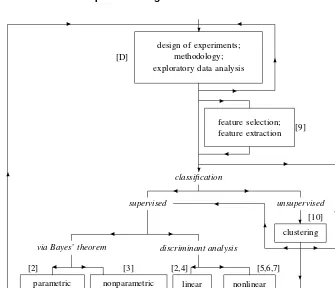
The techniques of Chapters 9 and 10 may be described as methods of exploratory data analysis or preprocessing (and as such would usually be carried out prior to the supervised classification techniques of Chapters 2–7, although they could, on occasion, be post-processors of supervised techniques). Chapter 9 addresses feature selection and feature extraction – the procedures for obtaining a reduced set of variables characterising the original data. Such procedures are often an integral part of classifier design and it is somewhat artificial to partition the pattern recognition problem into separate processes of feature extraction and classification. However, feature extraction may provide insights into the data structure and the type of classifier to employ; thus, it is of interest in its own right. Chapter 10 considers unsupervised classification orclustering– the process of grouping individuals in a population to discover the presence of structure; its engineering application is to vector quantisation for image and speech coding.
Finally, Chapter 11 addresses some important diverse topics including model selec-tion. Appendices largely cover background material and material appropriate if this book is used as a text for a ‘conversion course’: measures of dissimilarity, estimation, linear algebra, data analysis and basic probability.
The websitewww.statistical-pattern-recognition.netcontains refer-ences and links to further information on techniques and applications.
Notation
Some of the more commonly used notation is given below. I have used some notational conveniences. For example, I have tended to use the same symbol for a variable as well as a measurement on that variable. The meaning should be obvious from the context. Also, I denote the density function ofxas p.x/andyas p.y/, even though the functions differ. A vector is denoted by a lower-case quantity in bold face, and a matrix by upper case.
p number of variables
C number of classes
n number of measurements
ni number of measurements in classi
!i label for classi
X1; : : : ;Xp prandom variables
x1; : : : ;xp measurements on variables X1; : : : ;Xp x D .x1; : : : ;xp/T measurement vector
X D [x1; : : : ;xn]T nðpdata matrix X D
2
6 4
x11 : : : x1p ::
: : :: ::: xn1 : : : xnp
3
7 5
P.x/ D prob.X1x1; : : : ;Xpxp/ p.x/ D @P=@x
p.!i/ prior probability of classi
µ D R
xp.x/dx population mean
µi D R
xp.x/dx mean of classi;i D1; : : : ;C
mD.1=n/PnrD1xr sample mean
mi D.1=ni/PnrD1zirxr sample mean of classi;iD1; : : : ;C zir D1 ifxr 2!i;0 otherwise
ni Dnumber of patterns in!i DPnrD1zir O
D 1nPnrD1.xr m/.xr m/T sample covariance matrix (maximum likelihood estimate)
n=.n1/O sample covariance matrix
xviii NOTATION
O
i D .1=ni/PnjD1zi j.xjmi/.xj mi/T sample covariance matrix of classi (maximum likelihood estimate)
Si D nini1Oi sample covariance matrix of classi
(unbiased estimate) SW D PCiD1
ni
nOi pooled within-class sample
covariance matrix
S D nCn SW pooled within-class sample
covariance matrix (unbiased estimate) SB D PCiD1nin.mi m/.mi m/
T sample between-class matrix SBCSW D O
jjAjj2DP i jA2i j
N.m;/ normal distribution, mean; m
covariance matrix
E[YjX] expectation ofY given X
I. / =1 if =trueelse 0
1
Introduction to statistical pattern
recognition
Overview
Statistical pattern recognition is a term used to cover all stages of an investigation from problem formulation and data collection through to discrimination and clas-sification, assessment of results and interpretation. Some of the basic terminology is introduced and two complementary approaches to discrimination described.
1.1
Statistical pattern recognition
1.1.1
Introduction
This book describes basic pattern recognition procedures, together with practical appli-cations of the techniques on real-world problems. A strong emphasis is placed on the statistical theory of discrimination, but clustering also receives some attention. Thus, the subject matter of this book can be summed up in a single word: ‘classification’, both supervised (using class information to design a classifier – i.e. discrimination) and unsupervised (allocating to groups without class information – i.e. clustering).
Pattern recognition as a field of study developed significantly in the 1960s. It was very much an interdisciplinary subject, covering developments in the areas of statis-tics, engineering, artificial intelligence, computer science, psychology and physiology, among others. Some people entered the field with a real problem to solve. The large numbers of applications, ranging from the classical ones such as automatic character recognition and medical diagnosis to the more recent ones indata mining(such as credit scoring, consumer sales analysis and credit card transaction analysis), have attracted con-siderable research effort, with many methods developed and advances made. Other re-searchers were motivated by the development of machines with ‘brain-like’ performance, that in some way could emulate human performance. There were many over-optimistic and unrealistic claims made, and to some extent there exist strong parallels with the
2 Introduction to statistical pattern recognition
growth of research on knowledge-based systems in the 1970s and neural networks in the 1980s.
Nevertheless, within these areas significant progress has been made, particularly where the domain overlaps with probability and statistics, and within recent years there have been many exciting new developments, both in methodology and applications. These build on the solid foundations of earlier research and take advantage of increased compu-tational resources readily available nowadays. These developments include, for example, kernel-based methods and Bayesian computational methods.
The topics in this book could easily have been described under the term machine learningthat describes the study of machines that can adapt to their environment and learn from example. The emphasis in machine learning is perhaps more on computationally intensive methods and less on a statistical approach, but there is strong overlap between the research areas of statistical pattern recognition and machine learning.
1.1.2
The basic model
Since many of the techniques we shall describe have been developed over a range of diverse disciplines, there is naturally a variety of sometimes contradictory terminology. We shall use the term ‘pattern’ to denote thep-dimensional data vectorxD.x1; : : : ;xp/T of measurements (T denotes vector transpose), whose componentsxi are measurements of the features of an object. Thus the features are the variables specified by the investigator and thought to be important for classification. In discrimination, we assume that there existC groups or classes, denoted !1; : : : ; !C, and associated with each patternx is a categorical variablezthat denotes the class or group membership; that is, ifzDi, then the pattern belongs to!i,i 2 f1; : : : ;Cg.
Examples of patterns are measurements of an acoustic waveform in a speech recogni-tion problem; measurements on a patient made in order to identify a disease (diagnosis); measurements on patients in order to predict the likely outcome (prognosis); measure-ments on weather variables (for forecasting or prediction); and a digitised image for character recognition. Therefore, we see that the term ‘pattern’, in its technical meaning, does not necessarily refer to structure within images.
The main topic in this book may be described by a number of terms such aspattern classifier designordiscrimination orallocation rule design. By this we mean specifying the parameters of a pattern classifier, represented schematically in Figure 1.1, so that it yields the optimal (in some sense) response for a given pattern. This response is usually an estimate of the class to which the pattern belongs. We assume that we have a set of patterns of known classf.xi;zi/;i D1; : : : ;ng(the training or designset) that we use to design the classifier (to set up its internal parameters). Once this has been done, we may estimate class membership for an unknown patternx.
Stages in a pattern recognition problem 3
sensor
representation pattern
feature selector /extractor
feature pattern
classifier
decision
Figure 1.1 Pattern classifier
the suffering the patient is subjected to by each course of action and the risk of further complications.
Figure 1.1 grossly oversimplifies the pattern classification procedure. Data may un-dergo several separate transformation stages before a final outcome is reached. These transformations (sometimes termed preprocessing, feature selection or feature extraction) operate on the data in a way that usually reduces its dimension (reduces the number of features), removing redundant or irrelevant information, and transforms it to a form more appropriate for subsequent classification. The termintrinsic dimensionality refers to the minimum number of variables required to capture the structure within the data. In the speech recognition example mentioned above, a preprocessing stage may be to transform the waveform to a frequency representation. This may be processed further to find formants (peaks in the spectrum). This is a feature extraction process (taking a possible nonlinear combination of the original variables to form new variables). Feature selection is the process of selecting a subset of a given set of variables.
Terminology varies between authors. Sometimes the term ‘representation pattern’ is used for the vector of measurements made on a sensor (for example, optical imager, radar) with the term ‘feature pattern’ being reserved for the small set of variables obtained by transformation (by a feature selection or feature extraction process) of the original vector of measurements. In some problems, measurements may be made directly on the feature vector itself. In these situations there is no automatic feature selection stage, with the feature selection being performed by the investigator who ‘knows’ (through experience, knowledge of previous studies and the problem domain) those variables that are important for classification. In many cases, however, it will be necessary to perform one or more transformations of the measured data.
In some pattern classifiers, each of the above stages may be present and identifiable as separate operations, while in others they may not be. Also, in some classifiers, the preliminary stages will tend to be problem-specific, as in the speech example. In this book, we consider feature selection and extraction transformations that are not application-specific. That is not to say all will be suitable for any given application, however, but application-specific preprocessing must be left to the investigator.
1.2
Stages in a pattern recognition problem
4 Introduction to statistical pattern recognition
1. Formulation of the problem: gaining a clear understanding of the aims of the investi-gation and planning the remaining stages.
2. Data collection: making measurements on appropriate variables and recording details of the data collection procedure (ground truth).
3. Initial examination of the data: checking the data, calculating summary statistics and producing plots in order to get a feel for the structure.
4. Feature selection or feature extraction: selecting variables from the measured set that are appropriate for the task. These new variables may be obtained by a linear or nonlinear transformation of the original set (feature extraction). To some extent, the division of feature extraction and classification is artificial.
5. Unsupervised pattern classification or clustering. This may be viewed as exploratory data analysis and it may provide a successful conclusion to a study. On the other hand, it may be a means of preprocessing the data for a supervised classification procedure. 6. Apply discrimination or regression procedures as appropriate. The classifier is
de-signed using a training set of exemplar patterns.
7. Assessment of results. This may involve applying the trained classifier to an indepen-denttest setof labelled patterns.
8. Interpretation.
The above is necessarily an iterative process: the analysis of the results may pose further hypotheses that require further data collection. Also, the cycle may be terminated at different stages: the questions posed may be answered by an initial examination of the data or it may be discovered that the data cannot answer the initial question and the problem must be reformulated.
The emphasis of this book is on techniques for performing steps 4, 5 and 6.
1.3
Issues
The main topic that we address in this book concerns classifier design: given a training set of patterns of known class, we seek to design a classifier that is optimal for the expected operating conditions (the test conditions).
Supervised versus unsupervised 5
(due to noise). If the degree of the polynomial is too low, the fitting error is large and the underlying variability of the curve is not modelled.
Thus, achieving optimal performance on the design set (in terms of minimising some error criterion perhaps) is not required: it may be possible, in a classification problem, to achieve 100% classification accuracy on the design set but thegeneralisation perfor-mance– the expected performance on data representative of the true operating conditions (equivalently, the performance on an infinite test set of which the design set is a sam-ple) – is poorer than could be achieved by careful design. Choosing the ‘right’ model is an exercise inmodel selection.
In practice we usually do not know what is structure and what is noise in the data. Also, training a classifier (the procedure of determining its parameters) should not be considered as a separate issue from model selection, but it often is.
A second point about the design of optimal classifiers concerns the word ‘optimal’. There are several ways of measuring classifier performance, the most common being error rate, although this has severe limitations. Other measures, based on the closeness of the estimates of the probabilities of class membership to the true probabilities, may be more appropriate in many cases. However, many classifier design methods usually optimise alternative criteria since the desired ones are difficult to optimise directly. For example, a classifier may be trained by optimising a squared error measure and assessed using error rate.
Finally, we assume that the training data are representative of the test conditions. If this is not so, perhaps because the test conditions may be subject to noise not present in the training data, or there are changes in the population from which the data are drawn (population drift), then these differences must be taken into account in classifier design.
1.4
Supervised versus unsupervised
There are two main divisions of classification:supervised classification (or discrimina-tion) andunsupervised classification(sometimes in the statistics literature simply referred to as classification or clustering).
In supervised classification we have a set of data samples (each consisting of mea-surements on a set of variables) with associated labels, the class types. These are used as exemplars in the classifier design.
6 Introduction to statistical pattern recognition
vehicle recognition, the data may be gathered by positioning vehicles on a turntable and making measurements from all aspect angles. In the practical application, a human may not be able to recognise an object reliably from its radar image, or the process may be carried out remotely.
In unsupervised classification, the data are not labelled and we seek to find groups in the data and the features that distinguish one group from another. Clustering techniques, described further in Chapter 10, can also be used as part of a supervised classification scheme by defining prototypes. A clustering scheme may be applied to the data for each class separately and representative samples for each group within the class (the group means, for example) used as the prototypes for that class.
1.5
Approaches to statistical pattern recognition
The problem we are addressing in this book is primarily one of pattern classifica-tion. Given a set of measurements obtained through observation and represented as a pattern vector x, we wish to assign the pattern to one of C possible classes !i, i D 1; : : : ;C. A decision rule partitions the measurement space into C regions i, i D1; : : : ;C. If an observation vector is in i then it is assumed to belong to class !i. Each region may be multiply connected – that is, it may be made up of several disjoint regions. The boundaries between the regionsi are thedecision boundaries or decision surfaces. Generally, it is in regions close to these boundaries that the high-est proportion of misclassifications occurs. In such situations, we may reject the pat-tern or withhold a decision until further information is available so that a classification may be made later. This option is known as the reject option and therefore we have CC1 outcomes of a decision rule (the reject option being denoted by !0) in aC-class problem.
In this section we introduce two approaches to discrimination that will be explored further in later chapters. The first assumes a knowledge of the underlying class-conditional probability density functions (the probability density function of the feature vectors for a given class). Of course, in many applications these will usually be unknown and must be estimated from a set of correctly classified samples termed the design or training set. Chapters 2 and 3 describe techniques for estimating the probability density functions explicitly.
The second approach introduced in this section develops decision rules that use the data to estimate the decision boundaries directly, without explicit calculation of the probability density functions. This approach is developed in Chapters 4, 5 and 6 where specific techniques are described.
1.5.1
Elementary decision theory
Approaches to statistical pattern recognition 7
Bayes decision rule for minimum error
ConsiderCclasses,!1; : : : ; !C, witha priori probabilities (the probabilities of each class occurring) p.!1/; : : : ;p.!C/, assumed known. If we wish to minimise the probability of making an error and we have no information regarding an object other than the class probability distribution then we would assign an object to class!j if
p.!j/ > p.!k/ kD1; : : : ;C; k6D j
This classifies all objects as belonging to one class. For classes with equal probabilities, patterns are assigned arbitrarily between those classes.
However, we do have anobservation vector ormeasurement vector x and we wish to assignx to one of the C classes. A decision rule based on probabilities is to assign xto class !j if the probability of class!j given the observationx, p.!jjx/, is greatest over all classes!1; : : : ; !C. That is, assignx to class!j if
p.!jjx/ > p.!kjx/ kD1; : : : ;C;k6D j (1.1) This decision rule partitions the measurement space intoCregions1; : : : ; Csuch that ifx2j thenx belongs to class!j.
The a posteriori probabilities p.!jjx/ may be expressed in terms of the a priori probabilities and the class-conditional density functions p.xj!i/using Bayes’ theorem (see Appendix E) as
p.!ijx/D
p.xj!i/p.!i/ p.x/
and so the decision rule (1.1) may be written: assignx to!j if
p.xj!j/p.!j/ > p.xj!k/p.!k/ kD1; : : : ;C;k6D j (1.2) This is known as Bayes’ rule forminimum error.
For two classes, the decision rule (1.2) may be written lr.x/D
p.xj!1/ p.xj!2/
> p.!2/ p.!1/
impliesx2class!1
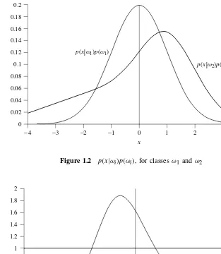
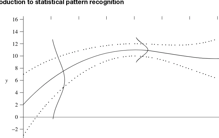
The functionlr.x/is thelikelihood ratio. Figures 1.2 and 1.3 give a simple illustration for a two-class discrimination problem. Class!1is normally distributed with zero mean and unit variance, p.xj!1/DN.xj0;1/(see Appendix E). Class!2 is anormal mixture (a weighted sum of normal densities)p.xj!2/D0:6N.xj1;1/C0:4N.xj1;2/. Figure 1.2 plots p.xj!i/p.!i/;iD1;2, where the priors are taken to be p.!1/D0:5, p.!2/D0:5. Figure 1.3 plots the likelihood ratiolr.x/and the threshold p.!2/=p.!1/. We see from this figure that the decision rule (1.2) leads to a disjoint region for class!2.
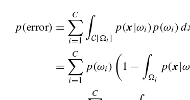
The fact that the decision rule (1.2) minimises the error may be seen as follows. The probability of making an error, p.error/, may be expressed as
p.error/D C X
iD1
8 Introduction to statistical pattern recognition
0
−4 −3 −2 −1 0 p(x|w
1)p(w
1)
p(x|w
2)p(w
2)
x
1 2 3 4
0.02 0.04 0.06 0.08 0.1 0.12 0.14 0.16 0.18 0.2
Figure 1.2 p.xj!i/p.!i/, for classes!1and!2
2
1.8
1.6
1.4
1.2
1
0.8
0.6
0.4
0.2
0
−4 −3 −2 −1 0 x
lr (x)
1 2 3 4
p(w
2)/p(w
1)
Figure 1.3 Likelihood function
where p.errorj!i/ is the probability of misclassifying patterns from class !i. This is given by
p.errorj!i/D Z
C[i]
p.xj!i/dx (1.4)
Approaches to statistical pattern recognition 9
may write the probability of misclassifying a pattern as
p.error/D C X
iD1
Z
C[i]
p.xj!i/p.!i/dx
D C X
iD1
p.!i/
1 Z
i
p.xj!i/dx
D1
C X
iD1
p.!i/ Z
i
p.xj!i/dx (1.5)
from which we see that minimising the probability of making an error is equivalent to maximising
C X
iD1
p.!i/ Z
i
p.xj!i/dx (1.6)
the probability of correct classification. Therefore, we wish to choose the regionsi so that the integral given in (1.6) is a maximum. This is achieved by selectingi to be the region for which p.!i/p.xj!i/is the largest over all classes and the probability of correct classification,c, is
cD Z
max
i p.!i/p.xj!i/dx (1.7) where the integral is over the whole of the measurement space, and the Bayes error is
eB D1 Z
max
i p.!i/p.
xj!i/dx (1.8)
This is illustrated in Figures 1.4 and 1.5. Figure 1.4 plots the two distributions p.xj!i/;i D 1;2 (both normal with unit variance and means š0:5), and Figure 1.5 plots the functions p.xj!i/p.!i/ where p.!1/ D 0:3, p.!2/ D 0:7. The Bayes
deci-sion boundary is marked with a vertical line at xB. The areas of the hatched regions in Figure 1.4 represent the probability of error: by equation (1.4), the area of the horizontal hatching is the probability of classifying a pattern from class 1 as a pattern from class 2 and the area of the vertical hatching the probability of classifying a pattern from class 2 as class 1. The sum of these two areas, weighted by the priors (equation (1.5)), is the probability of making an error.
Bayes decision rule for minimum error – reject option
10 Introduction to statistical pattern recognition
−4 −3 0
0.05 0.1 0.15 0.2
p(x|w
1) p(x|w
2) 0.25
0.3 0.35 0.4
−2 −1 0 xB
1 2 3 4
Figure 1.4 Class-conditional densities for two normal distributions
−4 −3 0
0.05 0.1 0.15 0.2
p(x|w
1)p(w
1)
p(x|w
2)p(w
2) 0.25
0.3
−2 −1 0 xB
1 2 3 4
Figure 1.5 Bayes decision boundary for two normally distributed classes with unequal priors
classifications are also converted into rejects. Here we consider the trade-offs between error rate and reject rate.
Firstly, we partition the sample space into two complementary regions: R, a reject region, and A, anacceptance or classification region. These are defined by
R Dnxj1 max
i p.!ijx/ >t/ o
ADnxj1 max
Approaches to statistical pattern recognition 11
0
−4 −3 −2 −1 0 R
A A
1 2 3 4
0.1 0.2 0.3 0.4 0.5 0.6 0.7 0.8 t 1 −t
0.9 1
p(w2|x)
p(w1|x)
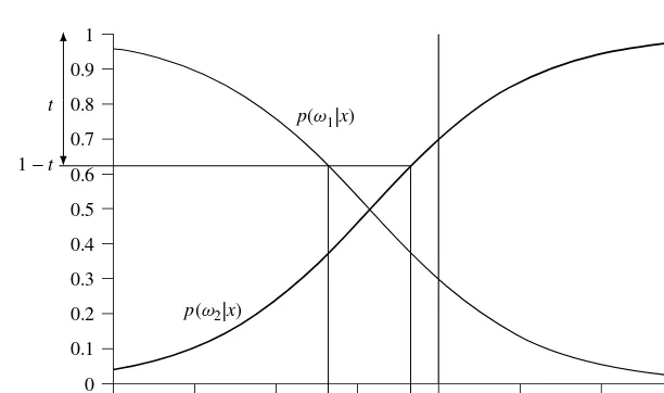
Figure 1.6 Illustration of acceptance and reject regions
wheret is a threshold. This is illustrated in Figure 1.6 using the same distributions as those in Figures 1.4 and 1.5. The smaller the value of the threshold t, the larger is the reject region R. However, if t is chosen such that
1t< 1 C
or equivalently,
t> C1 C
whereC is the number of classes, then the reject region is empty. This is because the minimum value which maxi p.!ijx/ can attain is 1=C (since 1 D PCiD1p.!ijx/ Cmaxi p.!ijx/), when all classes are equally likely. Therefore, for the reject option to be activated, we must havet .C1/=C.
Thus, if a patternx lies in the region A, we classify it according to the Bayes rule for minimum error (equation (1.2)). However, ifx lies in the region R, we rejectx.
The probability of correct classification,c.t/, is a function of the threshold,t, and is given by equation (1.7), where now the integral is over the acceptance region, A, only
c.t/D Z
A max
i ð
p.!i/p.xj!i/ Ł
dx
and the unconditional probability of rejecting a measurementx,r, also a function of the thresholdt, is
r.t/D Z
R
12 Introduction to statistical pattern recognition
Therefore, the error rate, e (the probability of accepting a point for classification and incorrectly classifying it), is
e.t/D Z
A
.1 max
i p.!ijx//p.x/dx D1c.t/r.t/
Thus, the error rate and reject rate are inversely related. Chow (1970) derives a simple functional relationship betweene.t/andr.t/which we quote here without proof. Know-ingr.t/over the complete range oft allowse.t/to be calculated using the relationship
e.t/D Z t
0
s dr.s/ (1.10)
The above result allows the error rate to be evaluated from the reject function for the Bayes optimum classifier. The reject function can be calculated using unlabelled data and a practical application is to problems where labelling of gathered data is costly.
Bayes decision rule for minimum risk
In the previous section, the decision rule selected the class for which the a posteriori probability, p.!jjx/, was the greatest. This minimised the probability of making an error. We now consider a somewhat different rule that minimises an expected loss or risk. This is a very important concept since in many applications the costs associated with misclassification depend upon the true class of the pattern and the class to which it is assigned. For example, in a medical diagnosis problem in which a patient has back pain, it is far worse to classify a patient with severe spinal abnormality as healthy (or having mild back ache) than the other way round.
We make this concept more formal by introducing a loss that is a measure of the cost of making the decision that a pattern belongs to class!i when the true class is !j. We define a loss matrixwith components
½j i Dcost of assigning a patternx to!i when x2!j
In practice, it may be very difficult to assign costs. In some situations,½may be measured in monetary units that are quantifiable. However, in many situations, costs are a combi-nation of several different factors measured in different units –money, time, quality of life. As a consequence, they may be the subjective opinion of an expert. Theconditional risk of assigning a patternx to class!i is defined as
li.x/D C X
jD1
½j ip.!jjx/
The average risk over regioni is
ri D Z
i
li.x/p.x/dx
D Z
i C X
jD1
Approaches to statistical pattern recognition 13
and the overall expected cost orrisk is
rD C X
iD1
ri D C X
iD1
Z
i C X
jD1
½j ip.!jjx/p.x/dx (1.11)
The above expression for the risk will be minimised if the regionsi are chosen such that if
C X
jD1
½j ip.!jjx/p.x/ C X
jD1
½j kp.!jjx/p.x/ kD1; : : : ;C (1.12)
then x 2 i. This is the Bayes decision rule for minimum risk, with Bayes risk, rŁ, given by
rŁD Z
x iDmin1;:::;C C X
jD1
½j ip.!jjx/p.x/dx
One special case of the loss matrixis theequal costloss matrix for which
½i j D ²
1 i 6D j 0 i D j
Substituting into (1.12) gives the decision rule: assignx to class!i if C
X
jD1
p.!jjx/p.x/p.!ijx/p.x/ C X
jD1
p.!jjx/p.x/p.!kjx/p.x/ kD1; : : : ;C
that is,
p.xj!i/p.!i/½ p.xj!k/p.!k/ kD1; : : : ;C
implies thatx2 class!i; this is the Bayes rule for minimum error.
Bayes decision rule for minimum risk – reject option
As with the Bayes rule for minimum error, we may also introduce a reject option, by which the reject region, R, is defined by
RDnxþþ þmini l
i.x/ >to
wheret is a threshold. The decision is to accept a patternx and assign it to class!i if
li.x/D min j l
j.
x/t
and to rejectx if
li.x/D min j l
14 Introduction to statistical pattern recognition
This decision is equivalent to defining a reject region0with a constant conditional risk
l0.x/Dt
so that the Bayes decision rule is: assignx to class!i if
li.x/lj.x/ j D0;1; : : : ;C
with Bayes risk
rŁD Z
R
t p.x/dxC Z
A min iD1;:::;C
C X
jD1
½j ip.!jjx/p.x/dx (1.13)
Neyman–Pearson decision rule
An alternative to the Bayes decision rules for a two-class problem is the Neyman–Pearson test. In a two-class problem there are two possible types of error that may be made in the decision process. We may classify a pattern of class!1as belonging to class!2or
a pattern from class!2 as belonging to class!1. Let the probability of these two errors
bež1 andž2respectively, so that
ž1D
Z
2
p.xj!1/dxDerror probability of Type I
and
ž2D
Z
1
p.xj!2/dxDerror probability of Type II
The Neyman–Pearson decision rule is to minimise the errorž1subject tož2being equal
to a constant,ž0, say.
If class !1 is termed the positive class and class !2 the negative class, then ž1
is referred to as the false negative rate, the proportion of positive samples incorrectly assigned to the negative class; ž2 is the false positive rate, the proportion of negative
samples classed as positive.
An example of the use of the Neyman–Pearson decision rule is in radar detection where the problem is to detect a signal in the presence of noise. There are two types of error that may occur; one is to mistake noise for a signal present. This is called afalse alarm. The second type of error occurs when a signal is actually present but the decision is made that only noise is present. This is amissed detection. If !1 denotes the signal
class and !2 denotes the noise then ž2 is the probability of false alarm and ž1 is the
probability of missed detection. In many radar applications, a threshold is set to give a fixed probability of false alarm and therefore the Neyman–Pearson decision rule is the one usually used.
We seek the minimum of
r D Z
2
p.xj!1/dxC¼
²Z
1
p.xj!2/dxž0
Approaches to statistical pattern recognition 15
where¼is a Lagrange multiplier1 andž0is the specified false alarm rate. The equation
may be written
rD.1¼ž0/C
Z
1
f¼p.xj!2/dxp.xj!1/dxg
This will be minimised if we choose1 such that the integrand is negative, i.e.
if¼p.xj!2/p.xj!1/ <0; thenx21
or, in terms of the likelihood ratio,
if p.xj!1/ p.xj!2/
> ¼; thenx21 (1.14)
Thus the decision rule depends only on the within-class distributions and ignores the a priori probabilities.
The threshold¼is chosen so that
Z
1
p.xj!2/dxDž0;
the specified false alarm rate. However, in general ¼cannot be determined analytically and requires numerical calculation.
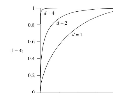
Often, the performance of the decision rule is summarised in a receiver operating characteristic (ROC) curve, which plots the true positive against the false positive (that is, the probability of detection (1ž1DR1 p.xj!1/dx) against the probability of false
alarm (ž2DR
1 p.xj!2/dx)) as the threshold¼is varied. This is illustrated in Figure 1.7
for the univariate case of two normally distributed classes of unit variance and means separated by a distance,d. All the ROC curves pass through the.0;0/and.1;1/points and as the separation increases the curve moves into the top left corner. Ideally, we would like 100% detection for a 0% false alarm rate; the closer a curve is to this the better.
For the two-class case, the minimum risk decision (see equation (1.12)) defines the decision rules on the basis of the likelihood ratio (½i i D0):
if p.xj!1/ p.xj!2/
>½21p.!2/ ½12p.!1/
; thenx 21 (1.15)
The threshold defined by the right-hand side will correspond to a particular point on the ROC curve that depends on the misclassification costs and the prior probabilities.
In practice, precise values for the misclassification costs will be unavailable and we shall need to assess the performance over a range of expected costs. The use of the ROC curve as a tool for comparing and assessing classifier performance is discussed in Chapter 8.
16 Introduction to statistical pattern recognition
0 0
d= 1 d= 2 d= 4
0.2 0.4 0.6 0.8 1
0.2 0.4 0.6 0.8 1
1 1 − ∋
2 ∋
Figure 1.7 Receiver operating characteristic for two univariate normal distributions of unit vari-ance and separationd; 1ž1D
R
1p.xj!1/dxis the true positive (the probability of detection)
andž2D
R
1p.xj!2/dx is the false positive (the probability of false alarm)
Minimax criterion
The Bayes decision rules rely on a knowledge of both the within-class distributions and the prior class probabilities. However, situations may arise where the relative frequencies of new objects to be classified are unknown. In this situation aminimax procedure may be employed. The name minimax is used to refer to procedures for which either the maximum expected lossorthe maximum of the error probability is a minimum. We shall limit our discussion below to the two-class problem and the minimum error probability procedure.
Consider the Bayes rule for minimum error. The decision regions 1 and 2 are
defined by
p.xj!1/p.!1/ > p.xj!2/p.!2/impliesx21 (1.16)
and the Bayes minimum error,eB, is
eB Dp.!2/
Z
1
p.xj!2/dxCp.!1/
Z
2
p.xj!1/dx (1.17)
where p.!2/D1p.!1/.
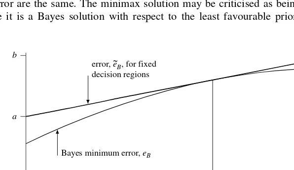
Forfixed decision regions 1 and2,eB is a linear function of p.!1/(we denote
this function eQB) attaining its maximum on the region [0;1] either at p.!1/ D 0 or
p.!1/D1. However, since the regions1and2are also dependent on p.!1/through
the Bayes decision criterion (1.16), the dependency ofeB on p.!1/is more complex,
and not necessarily monotonic.
Approaches to statistical pattern recognition 17
must be greater than the minimum error. Therefore, the optimum curve touches the line at a tangent at p1Łand is concave down at that point.
The minimax procedure aims to choose the partition 1, 2, or equivalently the
value of p.!1/ so that the maximum error (on a test set in which the values of p.!i/ are unknown) is minimised. For example, in thefigure, if the partition were chosen to correspond to the value p1Łof p.!1/, then the maximum error which could occur would
be a value ofb if p.!1/were actually equal to unity. The minimax procedure aims to
minimise this maximum value, i.e. minimise
maxfQeB.0/;eBQ .1/g
or minimise
max ²Z
2
p.xj!1/dx;
Z
1
p.xj!2/dx
¦
This is a minimum when
Z
2
p.xj!1/dxD
Z
1
p.xj!2/dx (1.18)
which is whenaDb in Figure 1.8 and the lineeQB.p.!1//is horizontal and touches the
Bayes minimum error curve at its peak value.
Therefore, we choose the regions1and2so that the probabilities of the two types
of error are the same. The minimax solution may be criticised as being over-pessimistic since it is a Bayes solution with respect to the least favourable prior distribution. The
0.0
Bayes minimum error, eB a
b
p(w
1) 1.0
p1* error, eB, for fixed
decision regions ~
18 Introduction to statistical pattern recognition
strategy may also be applied to minimising the maximum risk. In this case, the risk is
Z
1
[½11p.!1jx/C½21p.!2jx/]p.x/dxC
Z
2
[½12p.!1jx/C½22p.!2jx/]p.x/dx
Dp.!1/
½11C.½12½11/
Z
2
p.xj!1/dx
½
Cp.!2/
½22C.½21½22/
Z
1
p.xj!2/dx
½
and the boundary must therefore satisfy
½11½22C.½12½11/
Z
2
p.xj!1/dx.½21½22/
Z
1
p.xj!2/dxD0
For½11D½22 and½21D½12, this reduces to condition (1.18).
Discussion
In this section we have introduced a decision-theoretic approach to classifying patterns. This divides up the measurement space into decision regions and we have looked at various strategies for obtaining the decision boundaries. The optimum rule in the sense of minimising the error is the Bayes decision rule for minimum error. Introducing the costs of making incorrect decisions leads to the Bayes rule for minimum risk. The theory developed assumes that the a priori distributions and the class-conditional distributions are known. In a real-world task, this is unlikely to be so. Therefore approximations must be made based on the data available. We consider techniques for estimating distribu-tions in Chapters 2 and 3. Two alternatives to the Bayesian decision rule have also been described, namely the Neyman–Pearson decision rule (commonly used in signal process-ing applications) and the minimax rule. Both require knowledge of the class-conditional probability density functions. The receiver operating characteristic curve characterises the performance of a rule over a range of thresholds of the likelihood ratio.
We have seen that the error rate plays an important part in decision-making and classifier performance assessment. Consequently, estimation of error rates is a problem of great interest in statistical pattern recognition. For given fixed decision regions, we may calculate the probability of error using (1.5). If these decision regions are chosen according to the Bayes decision rule (1.2), then the error is the Bayes error rate or optimal error rate. However, regardless of how the decision regions are chosen, the error rate may be regarded as a measure of a given decision rule’s performance.
The Bayes error rate (1.5) requires complete knowledge of the class-conditional den-sity functions. In a particular situation, these may not be known and a classifier may be designed on the basis of a training set of samples. Given this training set, we may choose to form estimates of the distributions (using some of the techniques discussed in Chapters 2 and 3) and thus, with these estimates, use the Bayes decision rule and estimate the error according to (1.5).
Approaches to statistical pattern recognition 19
1.5.2
Discriminant functions
In the previous subsection, classification was achieved by applying the Bayesian decision rule. This requires knowledge of the class-conditional density functions, p.xj!i/(such as normal distributions whose parameters are estimated from the data– see Chapter 2), or nonparametric density estimation methods (such as kernel density estimation – see Chapter 3). Here, instead of making assumptions about p.xj!i/, we make assumptions about the forms of thediscriminant functions.
A discriminant function is a function of the patternxthat leads to a classification rule. For example, in a two-class problem, a discriminant functionh.x/is a function for which
h.x/ >k)x2!1 <k)x2!2
(1.19)
for constantk. In the case of equality (h.x/Dk), the patternxmay be assigned arbitrarily to one of the two classes. An optimal discriminant function for the two-class case is
h.x/D p.xj!1/ p.xj!2/
with k D p.!2/=p.!1/. Discriminant functions are not unique. If f is a monotonic
function then
g.x/D f.h.x// >k0)x2!1
g.x/D f.h.x// <k0)x2!2
wherek0D f.k/leads to the same decision as (1.19).
In theC-group case we defineC discriminant functions gi.x/such that
gi.x/ >gj.x/)x2!i jD1; : : : ;C; j 6Di
That is, a pattern is assigned to the class with the largest discriminant. Of course, for two classes, a single discriminant function
h.x/Dg1.x/g2.x/
withkD0 reduces to the two-class case given by (1.19). Again, we may define an optimal discriminant function as
gi.x/D p.xj!i/p.!i/
leading to the Bayes decision rule, but as we showed for the two-class case, there are other discriminant functions that lead to the same decision.
20 Introduction to statistical pattern recognition
particular functional form whose parameters are adjusted by a training procedure. Many different forms of discriminant function have been considered in the literature, varying in complexity from the linear discriminant function (in whichg is a linear combination of thexi) to multiparameter nonlinear functions such as the multilayer perceptron.
Discrimination may also be viewed as a problem in regression (see Section 1.6) in which the dependent variable, y, is a class indicator and the regressors are the pattern vectors. Many discriminant function models lead to estimates of E[yjx], which is the aim of regression analysis (though in regression y is not necessarily a class indicator). Thus, many of the techniques we shall discuss for optimising discriminant functions apply equally well to regression problems. Indeed, as wefind with feature extraction in Chapter 9 and also clustering in Chapter 10, similar techniques have been developed under different names in the pattern recognition and statistics literature.
Linear discriminant functions
First of all, let us consider the family of discriminant functions that are linear combina-tions of the components ofxD.x1; : : : ;xp/T,
g.x/DwTxCw0D
p X
iD1
wixiCw0 (1.20)
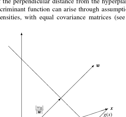
This is a linear discriminant function, a complete specification of which is achieved by prescribing the weight vector w and threshold weight w0. Equation (1.20) is the
equation of a hyperplane with unit normal in the direction of w and a perpendicular distancejw0j=jwjfrom the origin. The value of the discriminant function for a patternx
is a measure of the perpendicular distance from the hyperplane (see Figure 1.9). A linear discriminant function can arise through assumptions of normal distributions for the class densities, with equal covariance matrices (see Chapter 2). Alternatively,
origin g< 0 hyperplane, g= 0 g> 0
g(x)
Approaches to statistical pattern recognition 21
without making distributional assumptions, we may require the form of the discriminant function to be linear and determine its parameters (see Chapter 4).
A pattern classifier employing linear discriminant functions is termed alinear machine (Nilsson, 1965), an important special case of which is theminimum-distance classifier or nearest-neighbour rule. Suppose we are given a set of prototype points p1; : : : ;pC, one for each of the C classes !1; : : : ; !C. The minimum-distance classifier assigns a
patternxto the class!i associated with the nearest pointpi. For each point, the squared Euclidean distance is
jxpij2DxTx2xTpiCpiTpi
and minimum-distance classification is achieved by comparing the expressionsxTp i
1
2pTi pi and selecting the largest value. Thus, the linear discriminant function is gi.x/DwTi xCwi0
where
wi Dpi wi0D 12jpij2
Therefore, the minimum-distance classifier is a linear machine. If the prototype points,
pi, are the class means, then we have the nearest class mean classifier. Decision re-gions for a minimum-distance classifier are illustrated in Figure 1.10. Each boundary is the perpendicular bisector of the lines joining the prototype points of regions that are contiguous. Also, note from thefigure that the decision regions are convex (that is, two arbitrary points lying in the region can be joined by a straight line that lies entirely within the region). In fact, decision regions of a linear machine are always convex. Thus, the two class problems, illustrated in Figure 1.11, although separable, cannot be separated by a linear machine. Two generalisations that overcome this difficulty are piecewise linear discriminant functions and generalised linear discriminant functions.
Piecewise linear discriminant functions
This is a generalisation of the minimum-distance classifier to the situation in which there is more than one prototype per class. Suppose there areni prototypes in class!i,
p1i; : : : ;pnii ;i D1; : : : ;C. We define the discriminant function for class!i to be
gi.x/D max jD1;:::;ni
gij.x/
wheregij is a subsidiary discriminant function, which is linear and is given by
gij.x/DxTpij12p
j i T
pij j D1; : : : ;ni;i D1; : : : ;C
22 Introduction to statistical pattern recognition ž ž ž ž p1 p2 p3 p4
Figure 1.10 Decision regions for a minimum-distance classifier
ž ž ž ž ž ž ž ž ž ž Š Š Š Š Š Š Š Š Š Š Š Š ŠŠ (a) ž ž ž ž ž ž Š Š Š Š Š ž ž ž ž žžž (b)
Figure 1.11 Groups not separable by a linear discriminant
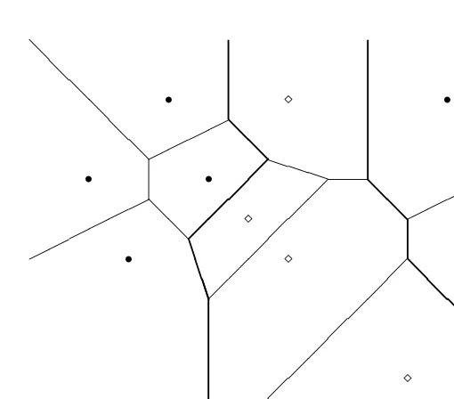
the Dirichlet tessellation of the space. When each pattern in the training set is taken as a prototype vector, then we have the nearest-neighbour decision rule of Chapter 3. This discriminant function generates a piecewise linear decision boundary (see Figure 1.12).
Rather than using the complete design set as prototypes, we may use a subset. Methods of reducing the number of prototype vectors (edit and condense) are described in Chapter 3, along with the nearest-neighbour algorithm. Clustering schemes may also be employed.
Generalised linear discriminant function
Ageneralised linear discriminant function, also termed aphi machine (Nilsson, 1965), is a discriminant function of the form
g.x/DwTφCw0
whereφ D .1.x/; : : : ;φD.x//T is a vector function of x. If D D p, the number of variables, andi.x/Dxi, then we have a linear discriminant function.
Approaches to statistical pattern recognition 23 ž ž ž ž ž ž Š Š Š Š
Figure 1.12 Dirichlet tessellation (comprising nearest-neighbour regions for a set of prototypes) and the decision boundary (thick lines) for two classes
x2 x1 ž ž ž ž ž ž ž Š Š Š Š Š Š Š Š Š 2 1 ž ž ž ž ž ž ž Š Š Š Š Š Š Š Š Š
Figure 1.13 Nonlinear transformation of variables may permit linear discrimination
if we make the transformation
1.x/Dx12 2.x/Dx2
then the classes can be separated in the -space by a straight line. Similarly, disjoint classes can be transformed into a-space in which a linear discriminant function could separate the classes (provided that they are separable in the original space).
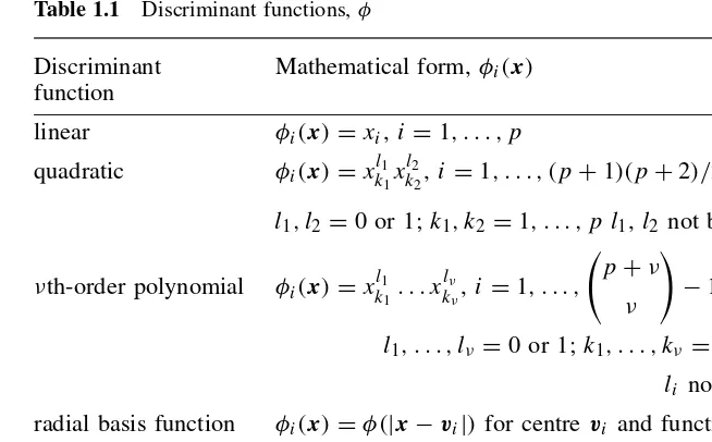
The problem, therefore, is simple. Make a good choice for the functions i.x/, then use a linear discriminant function to separate the classes. But, how do we choose i? Specific examples are shown in Table 1.1.
24 Introduction to statistical pattern recognition
Table 1.1 Discriminant functions,
Discriminant Mathematical form,i.x/ function
linear i.x/Dxi,iD1; : : : ;p
quadratic i.x/Dxkl11xkl22,iD1; : : : ; .pC1/.pC2/=21 l1;l2D0 or 1;k1;k2D1; : : : ;p l1,l2 not both zero
¹th-order polynomial i.x/Dxkl11: : :xkl¹¹,i D1; : : : ; pC¹
¹ !
1
l1; : : : ;l¹ D0 or 1;k1; : : : ;k¹ D1; : : : ;p li not all zero radial basis function i.x/D .jxvij/for centrevi and function multilay