Quantitative Easing Program and Financial Market Volatility in Indonesia

(1)

Jejak Vol 10 (1) (2017): 80-89. DOI: http://dx.doi.org/10.15294/jejak.v10i1.9128

JEJAK

Journal of Economics and Policy http://journal.unnes.ac.id/nju/index.php/jejak

Quantitative Easing Program and Financial Market Volatility

in Indonesia

T. Muhd. Redha Vahlevi1_{, Harjum Muharam}2

1,2_{Faculty of Economic and Bussiness Faculty Diponegoro University}

Permalink/DOI: http://dx.doi.org/10.15294/jejak.v10i1.9128

Received: June 2016; Accepted: August 2016; Published: March 2017

Abstract

This research aims to examine the impact of the USD money supply during and before quantitative easing program towards financial market volatility in Indonesia which is proxied by variance of financial market index such as IHSG, Gold Price in IDR, and Exchange

Rate IDR/USD to find out the effect of the excess USD money supply on Indonesia’s financial market volatility. This reseacrh has used monthly time series data of M1 of USD, IHSG, IDR/USD Exchange Rate, and Gold Price from December 2008 to December 2013. TGACRH in this research is used to find out wheter the volatility or variance at previous time affects volatility of these financial market index at present time and assymetric information is exist in the financial market index. The result showed that there’s a difference between the effect of USD money supply to financial market index volatility in Indonesia during QE program and before QE program. Before and during QE program, USD money supply positively affects IDR/USD exchange rate volatiliy and IHSG volatility and negatively affects Gold Price volatility. During QE program, USD money supply negatively affects volatility of IDR/USD exchange rate and IHSG, and positively affects Gold Price volatility.

Key words: USD Money Supply, Financial Market Volatility, IHSG, Gold Price, IDR/USD Exchange Rate.

How to Cite: Vahlevi, T., & Muharam, H. (2017). Quantitative Easing Program and Financial Market Volatility in Indonesia. JEJAK: Jurnal Ekonomi Dan Kebijakan, 10(1), 80-89. doi:http://dx.doi.org/10.15294/jejak.v10i1.9128

_{Corresponding author :}

Address: Prof. Soedharto SH street, Tembalang, Semarang 50239

E-mail: hardjum@gmail.com

(2)

INTRODUCTION

Financial market risk is a systemic risk that have powerfull effect for banking industry and firm, if market risk is very uncertainty and have high volatility then banking industry and firms will struggle enough to manage that risk. Financial

institution’s ability to manage market risk effect will determine the Financial

institution’s financial performance, if they

could manage risk driver of financial market risk carefully then the their performace will be better. Financial market risk includes movement of interest rate, stock market index, comodity index, or exhange rates. In this day, commodity market and financial market is experiencing fast globalization (Salvatore, 2011). The economic condition among countries become more integrated and dependendabilty. World financial and commodity market be more integrated. There is so many factors that causing world market more integrated. The change in USD supply will impact world economy because its function as international currency. Liu (2013) argues that one reason why people care so much about QE of US is that US dollar serves

as both US national currency and a “world currency”. United States is one of

Indonesian’s trading partners. Monetary

policy and economic condition in that

country will affect Indonesian’s financial market. During financial crisis in United States (Subprime mortgage) Bank Indonesia

increased the Bank Indonesia’s interest rate, it

is proved that financial and monetary policy in United States affected financial and monetary policy in Indonesia.

Since January 2009, the Chairman of Federal Reserve, Ben Bernanke, has established easy money policy which namely quantitative easing. This is a policy which sets both of low interest rate and open market

purchase to excess money supply massively for solving recession, spurs investment growth, decreasing unemployment, etc. Purwantoro (2013) argues that low interest rate policy that established by the Fed will affects world economic where amount of dollars in this world is 60% which has been used as reserves in the various countries. About 75% from global import of other countries except United States also still use United States dollar. on the QE 1 The Fed purchases US$100 billion of each month of Mortgage Backed Securities and on QE 2, QE 3, and QE 4 The Fed purchases US$ 85 billion each month long-term asset to inject money on circulation (Sheriff, 2013). In past several months, the exchange rate condition of Rupiah toward U.S. dollar is more apprehensive about. Throughout 2013, exchange rate of rupiah toward U.S. dollar has been depreciated more than 10%. QE policy also affected IHSG, many funds from foreign investors which came from U.S. is drawing back and huge capital outflow occurs and crushing dollar reserves almost until touch $90 billion (stabilitas keuangan, 2013). Furthermore, according to Ariston (2012) Gold as a commodity product receive positive impact

from the Fed’s stimulus.

Many researchs on USD money supply impact on financial market before and during QE (Quantitative Easing) program were conducted such as, Srikanth and Kishor (2012) concluded that relative money supply(M3 of India – M2 of US) are one of the most significant variable in determining the USD/INR exchange rate. Artigas (2010) argues 1% change in money supply in the US dollar, the European Union and United Kingdom, India, and Turkey tend to correlate to an increment in the price of gold. The reseacrh

of Quantitative easing’s effect on exchange rates

in Asia was conducted by Liu (2013), she found that the tremendous increase in the supply of US dollars caused by QE results in passive

(3)

82 T. Muhd. Redha Vahlevi andHarjum Muharam, Quantitative Easing Program

Phavaskar et al (2013) argue that Extra liquidity through QEs, in a method similar to that of osmosis, often goes beyond domestic boundaries and flows to capital-parched emerging market (EM) economies, offering a higher return on investment. Ahmed & Zlate (2012) found statistically not significant effects of unconventional U.S. monetary policy expansion on total net inflows of capital into EMEs. Furthermore, Fernandes (2012) argues that Quantitative easing have positive impact on Gold. Based on the phenomenon above and studies above, then the concern of this research is to analyze the impact of USD money supply on the exchange rate volatility, IHSG volatility, and the gold price volatility.

High money supply policy from the Fed such as open market purchase and decrease reserve requirement will caused federal fund rate is lower (Krugman and Obstfeld, 2011). According to Mishkin (2009) in his theory of asset demand, the demand for Indonesian stock or bond will be higher if the interest rate in U.S below the Indonesia Interest rate. Siklos and Anusiewicz(1998) state that unexpected high growth M1 USD led to higher Canadian stocks price. Low growth in M1 US led to lower Canadian stocks price. And than Panyasombat (2012) said that quantitative easing in order to excess money supply with near zero interest rate causes the capital outflow from U.S. to major financial market includes SET and S&P 500 and causes its price hikes.

According to monetary approach theory, if the U.S. money supply higher than Indonesia, USD will depreciate against IDR. And During Quantitative Easing Program which is established in order to make extreme growth in USD money supply, IDR will be appreciate towards USD. Srikanth and Kishor

(2012) have found the effect of the USD money supply on India Rupee Exchange Rata against USD. Phavaskar, et al (2012) said that the tapering off quantitative easing program which was issued in order to reduce USD money supply has caused the currency of other countries depreciated.

Gold such as other comodities which its price will hike when money supply excess. The unproperly money growth will cause inflationary effect on other comodities, gold is one of them. Fernandes (2012) has found that there is a significant relationship between QE1 and Crude Oil, using a 95% Confidence level. Artigas, et al (2010) argue that 1% change in money supply in the US dollar, the European Union and United Kingdom, India, and Turkey tend to correlate to an increment in the price of gold by 0.9%, 0.5%, 0.7%, and 0.05%, respectively.

RESEARCH METHODS

Data used in this research are US M1, IHSG, IDR toward US Dollar Exchange Rate, and Gold Price that obtained from Statistika Ekonomi dan

Keuangan Indonesia, Federal Reserve.org and

(4)

research is to examine the volatility and abnormal respons towards volatility which would be seen and explained by variance of each dependent variable, the reason to use TGARCH is to find out the asymetric information effect on the impact of USD money supply to financial market volatility in Indonesia. But before we are doing the analysis by TGARCH, then the data have to be tested by using ACF test and Unit Root test for ensure that there is no problem in stationarity and autocorrelation, And then they are have to tested by ARCH-LM test for ensure there is an ARCH effect on them. then the models with lowest AIC and SIC value are preffered (Ariefianto, 2012). If them was fulfilled then the analysis model is suitable for use. Finally, the result will be tested by using t-test.

The T-GARCH Model which is used for this result is such as follow :

𝜃2

1-t = Variance Rupiah/USD Exchange Rate Variable in t-period

𝜃2

2-t = Variance IHSG Variable in t-period

𝜃2

t-1 = Conditional variance in the previous

Autocorrelation Function (ACF) and Partial ACF Test

Autocorrelation function (ACF) shows how the realization of a variable at t period have a relationship with the realization of variable at the past period. Researchers could use the graphic that is called corelogram by ploting ACF value. This Graphic is very useful as evalution tools on statistic process in a time series data (Ariefianto, 2013). The result of ACF and PACF on level test shows that all variables was decline slowly and not stationare. Because the ARIMA models is done with stationary condition. The series of all variables was stationared by using its first difference.

Unit Root Test

Stationarity test is the important thing in

time series data analysis. The test which isn’t

suitable will cause inaccuracy in model then the

it will cause the conclusion isn’t accurate. The

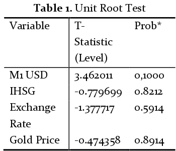
essentials of this procedure is to verificate the stationarity of the data generating process (DGP) (Ariefianto, 2013). The result of the initial data shows there is a problem about its stationarity. Therefore, data have to be transformed by using 1st difference for all the variable. The unit root test in this research is tested by Dickey-Fuller unit root test(1979) by computing statistic value and comparing it with its critical value. The result of this transformation process is such as on table 1.

(5)

Gold Price -0.474358 0.8914 Source : SEKI, Federal Reserve.org, and Goldpricefix.com

Table 2. Unit Root Test (First Difference)

Variable T-Statistic

Source : SEKI, Federal Reserve.org, and Goldpricefix.com

ARCH-LM Test

In addition ARCH testing in squared residual by correlogram, Engle has developed a test to find out heteroscedasticity in time series data named ARCH test (Widarjono 2013). The purpose of doing ARCH test is to find out the substance of ARCH on the models with lag 1 or 2. The result of this test is such as follow:

Table 3. ARCH-LM Test Result

Variable Prob. Chi-Square

IHSG (Lag 1) 0,0353

Exchange Rate (Lag 1) 0,0000 Gold Price (Lag 2) 0,0738

Source : Statistika Ekonomi dan Keuangan Indonesia, Federal Reserve.org, and Goldpricefix.com (processed data), 2014

Based on the figure above, alpha is lower than 10% with using lag 1 for IHSG and Exchange Rate and lag 2 for Gold Price. So, the null hypotesis which means that the residual variance is not constant or the model containts subtance of ARCH.

Threshold Generalized AutoRegressive

Conditional Heteroscedasticity (TGARCH)

Model and Hypotesis test

Because the volatility on financial assets like currency, stock market price, and gold price have volatility clustering, so this research uses the ARCH/GACRH model. GARCH model have a characteritic respon of volatility which symetric towards shock. In other words, along as the same of its intensity then the respons of volatility towards a shock is same too. The development of the next GARCH model acomodates the posibility of any asymetric volatility respons. There are two technique of asymetric GARCH, those are TGARCH (Threshold GARCH) and EGARCH (Exponential GARCH). The best model which is selected in this research is based on the lowest numbers in AIC(Akeike Info Criterion) and SIC(Schwarz criterion). And then, the hypotesis test on this research is T-test, EVIEWS could computed the p value from the statistic, so

this isn’t important to find out the critical value

on the table(t-table).

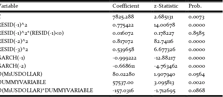
USD Money Supply and IHSG Volatility TGARCH Model

(6)

Table 4. TGARCH Variance Equation of IHSG

Variable Coefficient z-Statistic Prob.

C 7825.288 2.685131 0.0073

RESID(-1)^2 0.775422 14.00678 0.0000

RESID(-1)^2*(RESID(-1)<0) 0.016072 0.178227 0.8585

RESID(-2)^2 0.817072 82.74116 0.0000

RESID(-3)^2 0.539658 6.677326 0.0000

GARCH(-1) -0.999222 -12.88217 0.0000

GARCH(-2) -0.668611 -4.763462 0.0000

D(M1USDOLLAR) 80.02280 1.907940 0.0564

DUMMYVARIABLE 57537.00 3.095813 0.0020

D(M1USDOLLAR)*DUMMYVARIABLE -157.0316 -1.712695 0.0868

Source : eviews output

Because of the t significant of M1 USD variable is lower than alpha 10%, so Ha is accepted and Ho is rejected. And the regression equation (TGARCH) shows if money supply of USD excess about 1 billion, then it will impact IHSG volatility about Rp. 80,02. And this TGARCH model shows that there is a difference on the effect on IHSG volatility during quantitative easing program and before quantitative easing program, and the effect is significant because the p value of

dummy variable’s coefficient is lower than

10%, the model also presents that the excess USD money supply during quantitative easing program negatively affects the IHSG volatility with significant at alpha 10% or at 90% confidence level. And then, the IHSG TGARCH model shows that the volatility of IHSG at t time more explained by its ARCH1, ARCH2, ARCH3 it means that variances at previous time or at t-1, t-2, t-3 time has positive significant impact on IHSG volatility. Finally, the TGARCH model of IHSG shows that GARCH1, GARCH2 or conditional variance at previous time has negative

significant effect on IHSG volatility with

confidence level 99%. Then, the model shows that the bad news affects the IHSG volatility but

this effect isn’t significant because its p value is above 10%.

Krugman and Obstfeld (2011) was right, the extreme growth of USD causes interest rate on USA lower than before, so it will cause the capital outflow from USA to another country which asset in its currency gives higher return. During quantitative easing program, USD money supply has extremely growth, and USA has lower interest rate return than Indonesia, so the capital will flow from USA to Indonesia in order to seek the higher return.

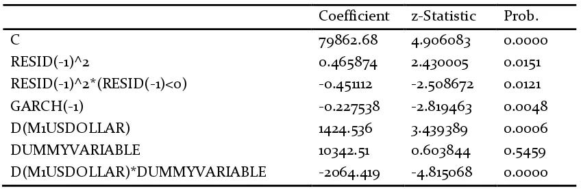
USD Money Supply and Exchange Rate Volatility TGARCH Model

(7)

Table 5. TGARCH Variance Equition of Exchange Rate

Coefficient z-Statistic Prob.

C 79862.68 4.906083 0.0000

RESID(-1)^2 0.465874 2.430005 0.0151

RESID(-1)^2*(RESID(-1)<0) -0.451112 -2.508672 0.0121

GARCH(-1) -0.227538 -2.819463 0.0048

D(M1USDOLLAR) 1424.536 3.439389 0.0006

DUMMYVARIABLE 10342.51 0.603844 0.5459

D(M1USDOLLAR)*DUMMYVARIABLE -2064.419 -4.815068 0.0000

Source : eviews output

Because of the p value of M1 USD’s coefficient is lower than alpha 1%, so Ho is accepted and Ha is rejected. And the regression equation (TGARCH) shows if money supply of USD excess about 1 billion, then it will positively impact Exchange Rate volatility about 1424,36 IDR/USD. And the dummy variable from this model indicates that the quantitative easing program which was established in order to excess money supply or liquidity in circulation has negative impact on the exchange rate and it is significant because the p value is lower than alpha 1% or it is significant with confidence level 1%. And then, exchange rate TGARCH model shows that the volatility of IDR/USD exchange rate at t time also explained by its ARCH1 with confidence level 5%, it means volatility of IDR/USD at t time is affected by its variance previous time or at t-1 time and its impact is significant with alpha 5%. The TGARCH model of IDR/USD exchange rate shows that GARCH1 has negative coefficient and its impact is significant with confidence level 1%, it means conditional variance at previous time has negative effect on IDR/USD exchange rate volatility. The TGARCH model also presents that the good news affects the IDR/USD exchange rate volatility rather than

bad news and this effect is significant at confidence level 95%.

This result is same as the research which did by Srikanth and Kishor (2012). They argue that exchange rates is affected by the relative money supply of domestic and foreign money supply. And furthermore, the nearly same result was found by Phavaskar (2012), he concluded that tapering off quantitative easing announcement which decreases USD money supply caused the depreciation. And this research result on IDR/USD exchange rate is not consistent with the monetary approach theory which states that the country which its currency has higher money supply growth than its demand will be depreciate againts the country which its money supply growth is lower or equal to its demand. The IDR/USD is positively affected by USD money supply, it means that the IDR/USD exchange rate is experienced depreciation not appreciation when USD money supply increases, so this research result is different from the monetary approach theory.

USD Money Supply and Gold Price Volatility TGARCH Model

(8)

Table 6. TGARCH of Gold Price

Variable Coefficient z-Statistic Prob.

C 168755.6 7.916507 0.0000

RESID(-1)^2*(RESID(-1)<0) -0.089621 -3.889804 0.0001

GARCH(-1) -0.755469 -4.062477 0.0000

D(M1USDOLLAR) -784.9959 -1.396113 0.1627

DUMMYVARIABLE 291890.5 4.519424 0.0000

D(M1USDOLLAR)*DUMMYVARIABLE 997.3184 1.490052 0.1362

Source: Eviews Output

Based on the estimation of the TGARCH model above, it could be seen that the M1 USD variable has a negative unsignificant impact on the gold price volatility. Then, t significant of M1 USD variable is higher than alpha 10%, so Ho is accepted and Ha is rejected. It means that there is a negatively significant impact of the M1 USD excessiveness on gold price volatility, and the regression equation (TGARCH) shows if money supply of USD excess about 1 billion, then it will affect gold price volatility about -784,99. And this TGARCH model shows that there is a difference on the effect on gold price volatility during quantitative easing program and before quantitative easing program, and the effect is unsignificant because the p value of dummy variable on M1 USD is higher than 10%. Furthermore, the TGARCH model of gold price shows that good news affects the gold price volatility rather than bad news, and its effect is significant at 10% confidence level, then TGARCH model shows that GARCH1 has negative value on its coefficient and it has p value 0,0000 with confidence level 99%, it means that conditonal variance at previous time affects the gold price volatility negatively and its effect is significant. And finally, the dummy variable of the model shows that money supply during quantitative easing program has positive impact the gold price volatility and this impact is unsignificant.

The result is different from the result which was found by Artigas, et al (2010). They conclude that the excess money supply growth in

U.S. affects the world’s gold price. And the same

result was found by Fernandes(2012). She argues that the quantitative easing program which is named by large scale assets purchasing in order to excess USD money supply extremely affects the gold price. Extreme USD money supply growth during Quantitative Easing Program causes the another asset more valuable because the USD value is experienced depreciation. And its inflationary effect causes the another asset and comodity such as gold has higher value than USD could not explain this research result before Quantitative Easing, but, when Quantitative Easing program, the USD money supply have a positive impact on gold price, it means that extreme USD money supply cause the new stationarity on gold price because it’s reducing the volatility on Gold Price Index.

CONCLUSION

Based on result of the data analysis and hypotesis testing from chapter IV, the conclusion of this research is such as follow :

(9)

Quantitative Easing program which excess the USD money supply has a negative impact on IHSG volatility. The hypothesis testing show that the t-significant is lower than alpha 10%, so the first is accepted. And then, the TGARCH model shows that the volatility of IHSG at t time is affected by its ARCH1, ARCH2, ARCH3 or variances at one period before, two period before, and three period before. Furthermore, the TGARCH model of IHSG presents that the volatility of IHSG at t time is also affected by its GARCH1 and GARCH2 or conditional variance at one period before and two period before. Finally TGACRH model of IHSG presents that bad news unsignificantly affects IHSG volatility . 2. Based on result of the hypothesis testing of

the impact of USD money supply towards IDR/USD exchange rate volatility that was mentioned on the previous chapter. It could be concluded that the USD money supply have a significant impact towards IDR/USD exchange rate volatility. The hypothesis testing show that the t-significant is 0.0006 which is lower than alpha 5%, so the second hypotesis is rejected because the impact of U.S. dollar money supply on IDR/USD Exchange Rate is positive. Quantitative easing program which excess USD money supply tremendously has negative impact on exchange rate volatility and during this program, exchange rate IDR/USD was experienced passive appreciation. And then, the TGARCH model shows that the volatility of IDR/USD exchange rate at t time is affected by its ARCH1 or variance at one period before. Furthermore, the TGARCH model of IDR/USD exchange rate presents that the volatility of IDR/USD at t time is also affected by its

GARCH1 or conditional variance at one period before. Finally, TGARCH model of IDR/USD exchange rate shows that good news has more impact than bad news on IDR/USD exchange rate volatility.

3. Based on result of the hypothesis testing of the impact of USD money supply towards gold price that was mentioned on the previous chapter. It could be concluded that the quantitative easing policy have an insignificant positive impact towards gold price volatility and USD money supply has negative impact toward gold price volatility

and it’s insignificant. The hypothesis testing

show that the t-significant is 0.1627 which is higher than alpha 10%, and the M1 USD negatively affects the gold price volatility, so the first hypothesis is rejected. Furthermore, the TGARCH model of gold price presents that the volatility of gold price at t time is also affected by its GARCH1 or conditional variance at one period before. Finally, TGARCH model of gold price shows that good news has more impact than bad news on gold price volatility.

REFERENCES

Ahmed, Shaghil and Andrei Zlate. 2012. “Capital Flows to

Emerging Market Economies : A Brave New

World ?”. International Finance Discussion Papers.

Board of Governors of the Federal Reserve System. Number 1081.

Ariefianto, M. Doddy. 2012. Ekonometrika. Jakarta: Erlangga.

Ariston. 2012. “Pengaruh Kebijakan Stimulus The Fed terhadap harga emas”. Http://www.kontan.com,

acessed on 30th January 2014.

Artigas, Juan, et al. 2010. “Linking Global Money Supply to

Gold and to Future

Inflation”. World Gold Trust Services.

Bessis, Joel. 2002. Risk Management in Banking. New York: Willey J. Finance.

Fernandes, Erica. 2012. “Quantitative Easing: A blessing or a

curse”. K.J. Somaiya Institute of Management Studies

(10)

Krugman, Paul R.and Maurice Obstfeld . 2011. International Economics. New York: Pearson Education.

Liu, Kai. 2013. “US Money Supply and China’s Economic

Fluctuation”. Journal of Economic. University of

Cambridge. U.K.

Liu, Yingxi. 2013. “Quantitative Easing: Reflections on

Practice and Theory” . World View of Political

Economy, Vol. 4. No. 3.

Mishkin, Frederic.S. 2009. Economic of Money, Banking and Financial Markets. New York: Pearson Education.

Mishkin, Frederic.S. 2013. Economic of Money, Banking and Financial Markets. New York: Pearson Education.

Panyasombat, Themaporn. 2012. “A Study of The Impact

of two U.S. Quantitative Easing Programs On

Major Financial Market”.

Phavaskar, Madho , et al. 2012. “Reverberation of QE

Tapering: A Global Assessment”. Financial

Technologi India.

Purwantoro, Nugroho., 2013, “Easy money Policy dari

The Fed”, Warta Ekonomi, 16 Juni 2013

Salvatore, Dominick. 2011. International Economics. New York: Willey J. New York.

Sheriff, Rasheed. 2013. “Impact of Possible Tapering of

Quantitatieve Easing to Emerging Frontier

Markets”. Kenanga Investment Corporation.

Siklos, Pierre and John Anusiewicz. 1998. “The Effect of

Canadian and U.S. M1 Announcement on Canadian

Financial Market”. Journal of Economic and

Bussiness. New York, 50:49-65.

Maram, Srikanth and Kishor, Braj, Exchange Rate Dynamics in Indian Foreign Exchange Market: An Empirical Investigation on the Movement of USD/INR (December 4, 2012). The IUP Journal of Applied Finance, Vol. 18, No. 4, October 2012, pp. 46-61.

Available at

SSRN: http://ssrn.com/abstract=2184743

Statistika Ekonomi dan Keuangan Indonesia. Januari 2003- Desember 2013. Jakarta: Bank Indonesia Techarongrojwong, Yaowaluk. 2013. “The Stock Market

Reaction to the U.S. Quantitative Easing Announcement : Evidence of the Emerging Stock

Market”. The Journal of American Academy of