Warehouse Selection for Storage of Finished Goods

(1)

Warehouse Selection for Storage of Finished Goods

Sarinah Sihombing STMT Trisakti stmt@indosat.net.id yoritupang@yahoo.com

Gires Firera STMT Trisakti stmt@indosat.net.id

ABSTRACT

In selecting a warehouse for storage of finished goods, from qualitative and quantitative data, aggregate value was obtained as a requirement to make choices and determine

costs.

Keyword: logistic, warehouse, analysis hierarchy process (AHP)

Introduction

Currently, almost all manufacturing companies have a warehouse, which gener

-ally serves as a temporary storage of goods

in each stage of the logistics process.

PT. Frisian Flag Indonesia (FFI) is a

manufacturing company that produces

healthy drinks such as powder and liquid milk with various other sub-products. In its operational activities, the FFI must al

-ways maintain the quality of the products it produces, especially the storage activities in the warehouse. The warehouse used for

temporary storage of the products as well as

a warehouse and distribution center is man

-aged by PT. YCH Indonesia. In addition to insufficient storage location, FFI also pays

attention to the hygiene or sterilization of

the warehouse environment and facilities that will be used to store all the finished products. It is being considered because the nature of the products requires special

treatment.

With the increasing number of new

products, followed by the addition of prod

-uct inventory in order to win the competi

-tion, FFI must be able to store the finished

products in a larger scale at the central

warehouse. However, due to the increase of additional inventory in the warehouse, FFI is looking for a new warehouse that can accommodate inventory with larger scale, better quality, and at a competitive cost.

Besides in Jakarta, FFI has other ware

-houses in other cities like in Surabaya, Se

-marang and Medan. It is aimed to make equal distributions of the product to be spread all over Indonesia. Of course, all the determinations and decisions on making warehousing services should be based on defined criteria.

This research used qualitative and quan

-titative data. Qualitative data is used for non-statistical analysis. Meanwhile, quan

(2)

-gistics managerss and the secondary data is

obtained from other parties related to the

research.

The measurement of the answer is based on Analytical Hierarchy Process method (AHP).

Analytical Hierarchy Process (AHP) is a systematic decision making method which was introduced by Thomas L. Saaty

during 1971-1975 when he was in Wharton

School. It is used if there are various crite

-ria of the decision making. There are some principals that need to be understood from the AHP method, namely: decomposition, comperative judgment, synthesis of prior

-ity, dan logical consistensy.

Furthermore, AHP also has a special concern about the deviations of consisten

-cy in the pairwise comparison matrix. First, the decision makers make a scoring on the relative importance between two elements qualitatively of “vertical (ci)” element with “horizontal (cj)” element in the pairwise

comparison matrix using the following for-mula: (Saaty, 1994).

Results and Disscusion

a. Rating the relative importance of two elements

...(1)

a = Pairwise Comparison matrix.

c_i,c_j,...,n = Elements (criteria) on pairwise

comparison matrix of a level in a hierar -chy.

w_i,w_j,...,w_n= The relative importance score

between the two elements of the

matrix of pairwise comparison

based on the interpretation of paired comparisons (attachment

IV appendix B.1)

After scoring the relative importance be

-tween elements, the inverse value is carried out to obtain the inverse score or reciprocal axiom, using the following formula:

b.Reciprocal axiom

a_ij = 1

a_ij ...(2)

a = Pairwise Comparison matrix

c

i,cj,...,n = Elements (criteria) on pairwise comparison matrix of a level in a hierarchy. The scoring was

performed to measure the con-sistency of the results of the

relative importance between elements scoring quantitatively. The results of these scoring is said to be perfect or consistent if it satisfies the following for -mula:

c. Consistancy Scoring

....(3)

a = Pairwise Comparison matrix.

n or z = The total of relative importance be

-tween elements (ci, cj, ck, ..., n) scoring and the inverse value (re

-ciprocal axiom) in each column of the Pairwise Comparison matrix or the Eigen values

w = priority score of pairwise comparison matrix.

This assessment was conducted to determine the validity of the priority score of pairwise comparison matrix. Thus obtained Zmax or Eigen value that meets the priority score in the pairwise comparison matrix. The

consistency of the indicators measured aij = wi/wj

(3)

through the Consistency Index (CI)

formulated as follow:

1. Counting the Consistensy Index value

...(4)

CI = Consistensy Index.

Z_max = the maximum Eigen value of the

pairwise comparison matrix n = the no of elements of pairwise

comparison matrix

AHP measures the entire consistency value using the Consistency Ratio (CR) as defined:

2.Counting the Consistency Ratio (CR)

...(5) CR = Consistensy Index (CI)

Random Consistensy Index *) RI score is the score of the Random Index issued by Oarkridge Laboratory in the form shown in table 1. n is the number of criteria

contained in the pairwise comparison ma-trix.

Determination of the Criteria of Each Warehouse Selection Priority

The decision makers should consider the following items before making the deci -sion:

1. Warehouse’s width; this is the first crite

-ria should be considered.

2. Fasilities; assessed only on the avail

-ability of pallets owned by the suppliers

and types of storage facilities on each

al-ternative which are racking and stacking blocks (bulk)

3. cost; assessed from the rental and ship -ping costs from the factory to the ware-house as well as the cost per pallet.

4. Location; assessed from the distance and travel time between factories and ware -houses

What being analyzed in this case is three warehouses with their own criteria, namely warehouse A, B, and C.

Table 2 is pairwise comparison matrix of the criteria of warehouse selection equiped with the relative importance score between elements and values of axioms Reciprocal based on the results of relative importance score between elements of decision mak

-ers value.

The table is the initial assessment done by comparing the vertical elements with

horizontal elements.

1. Warehouse’s width is more important

than facilities so it is weighted 3.

2. Cost is more important than warehouse’s

width so it is weighted 3.

3. Warehouse’s width is more important

than location so it is weighted 5.

4. Cost is more important than facilities so

it is weighted 5.

5. Facilities is more important than loca

-tion so it is weighted 3.

6. Cost is more important than location so it is weighted 5.

The matrix gave result to the total value for each column that is Eigen value (Z) of

the pairwise comparison matrix. Column

that has the smallest Eigen value will be

the highest priority score to the normalized matrix.

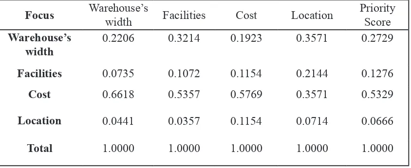
Table 3 refers to normalized matrix which was gained from the division of the pairwise comparison matrix and the Eigen value of each column. It shows the results of the perfect normalization calculations, as the total value of each column is 1.0000,

CI = Zmax – n

(4)

The comparison between alternative warehouses and warehouses’ width criterion

The first criterion is to perform pairwise comparisons for each alternative of warehouse’s width criterion. Filling the relative importance score of each alternative

against the warehouse’s width criterion is

done by using the result of the interviews done to the logistics managers, as seen on table 4.

The table is the initial assessment done by comparing the vertical elements with

horizontal elements.

a. Alternative Warehouse B is more impor

-tant than alternative Warehouse A, so it is weighted 3.

b. Alternative Warehouse C is much more important than alternative Warehouse A

so it is weighted 7.

c. Alternative Warehouse C is more impor

-tant than alternative Warehouse B so it is

weighted 5.

The matrix gave result to the total value for each column that is Eigen value (Z)

of the pairwise comparison matrix of the

warehouse’s width. Next is to make the normalized matrix as shown in table 5.

Table 5 refers to normalized matrix which was gained from the division of the

pairwise comparison matrix of warehouse’s

width criterion and the Eigen value of each

column. It shows the results of the perfect

normalization calculations, as the total val

-ue of each column is 1.0000. It also shows

the priority scores for each column.

After getting the priority score, the next is to test the consistency of the relative im

-portance assessment between elements by setting the value of Consistency Ratio (CR)



as well as the priority scores for each cri-terion

After getting the priority score, the next

is to test the consistency of the results of

relative importance score between elements by setting the value of Consistency Ratio (CR) through the following steps:

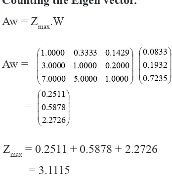
1. Counting the Eigen Vector Score.

Aw = Z_max.w It shows that each element (criterion)

contains the priority score of the ele-ment.

2.Counting the Consistency Index (CI).

CI = Z_max– n = 4.2847 – 4 n – 1 4 − 1

= 0.0949

3.Counting the Consistency Ratio (CR).

CR = CI = 0.0949 = 0.1055 RI 0,90

n is criteria compared. Based on table 1 RI

score for n = 4 is 0.90

The CR value gained from the calculation above is 0.1055. Because CR ≤ 0.10 then, there is no need to do the assessment revi

-sion because the priority score of each al

-ternative is consistent and valid

Determination of Alternative Priority toward Each Criterion

(5)



through the following steps: a. Counting the Eigen vector.

Aw = Zmax.W tains the priority score of the element. b.Counting Consistensy Index (CI).

CI = Z_max – n = 3.1115 – 3 = 0.0557 n – 1 3 – 1

c.Counting the Consistensy Ratio (CR).

CR = CI = 0.0557 = 0.0961 RI 0.58

n is criteria compared. Based on table 1 RI

score for n = 3 is 0.58

The CR value gained from the calculation above is 0.0961. Because CR ≤ 0.10 then, there is no need to do the assessment revi

-sion because the priority score of each al

-ternative is consistent and valid.

The Comparison between Alternative Warehouses and Facilities Criterion

The next process is to perform pairwise comparisons for each alternative against the facilities criterion. Filling the relative im

-portance score of each alternative against the facilities criterion is done by using the result of the interviews done to the logis

-tics managers like the steps taken before as shown in the matrix of table 6.



The matrix gave result to the total value for each column that is Eigen value (Z) of the

pairwise comparison matrix of the

facili-ties. Next is to make the normalized matrix as shown in table 7.

Table 7 refers to normalized matrix which was gained from the division of the pair -wise comparison matrix of facilities

crite-rion and the Eigen value of each column. It

shows the results of the perfect

normaliza-tion calculanormaliza-tions, as the total value of each column is 1.0000. It also shows the priority

scores for each column

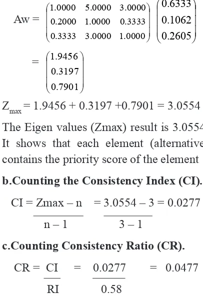
through the following steps: a.Counting the Eigen vector.

Aw = Z_max .w

Aw =

=

Z_max =1.5095 +0.9524+0.5988 = 3.0607 The Eigen values (Zmax) result is 3.0607. It shows that each element (alternative)

contains the priority score of the element. b.Counting the Consistency Index (CI).

CI = Zmax – n = 3.0607 – 3 = 0.0304 n – 1 3 – 1

c.Counting the Consistency Ratio (CR).

CR = CI = 0.0304 = 0.0523 RI 0.58

Based on the above calculation, the CR val

(6)



ue is 0.0523. Because CR ≤ 0.10 then, there is no need to do the assessment revision be

-cause the priority score of each alternative is consistent and valid.

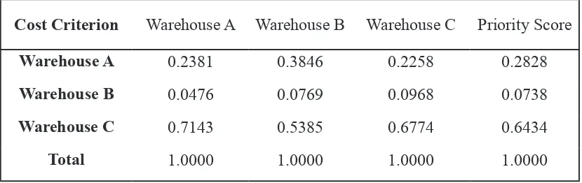
The comparison between Alternative Warehouses and Cost Criterion

The next process is to perform pairwise comparisons for each alternative against the criteria of cost. Filling the relative impor

-tance score of each alternative against the Cost criterion is done by using the result of the interviews done to the logistics manag

-ers and resulted in the matrix of table 8: The matrix gave result to the total value for each column that is Eigen value (Z) of

the pairwise comparison matrix of the cost.

Next is to make the normalized matrix as shown in table 9.

Table 9 refers to normalized matrix which was gained from the division of the pair -wise comparison matrix of cost criterion

and the Eigen value of each alternative. After getting the priority score, the next is to test the consistency of the relative im

through the following steps: a. Counting eigen vector value.

Aw = Z_max .w

Aw =

=

Z_max = 0.8662 + 0.2223 + 2.0083 = 3.0967 The Eigen values (Zmax) result is 3.0967. It shows that each element (alternative)

contains the priority score of the element



b.Counting the Consistency Index (CI).

CI = Zmax – n = 3.0967 – 3 = 0.0484 n – 1 3 − 1

c.Counting the Consistency Ratio (CR).

CR = CI = 0.0484 = 0.0834 RI 0.58

Based on the above calculation, the CR val

-ue is 0.0834. Because CR ≤ 0.10 then, there is no need to do the assessment revision be

-cause the priority score of each alternative is consistent and valid.

The Comparison between Alternative Warehouses and Location Criterion

Then, the process followed by pairwise comparisons for each alternative against

the criterion of location using the result

of the interviews to the logistics managers

so we get a pairwise comparison matrix as

seen on table 10.

The matrix gave result to the total value for each column that is Eigen value (Z) of the

pairwise comparison matrix of the location.

Next is to make the normalized matrix as shown in table 11.

Table 11 refers to normalized matrix which was gained from the division of the

pairwise comparison matrix of location

cri-terion and the Eigen value of each column.

It shows the results of the perfect

normal-ization calculations, as the total value of each column is 1.0000. It also shows the

priority scores for each column.

through the following steps:

a.Counting the Eigen Vector Score.

(7)

bigger than others that is 0.5829. Its width is 27,900 m2. It has 44,682 pallet capacity. Besides, it has Racking and Block Stacking (Bulk) facility, because it is located in Cibitung or 28 km from the factory, so it takes only one and half hour to get there.

The cost that needs to be prepared by the company is Rp 1,413,036,625 as the delivery cost from the factory to the warehouse is Rp 1,300,000 and the cost per pallet is Rp 31,625.

References

Arwani, A. 2009. Warehouse Check up.

Jakarta: PPM.

Heizer, J & Render, B. 2010. Manajemen

Operasi. Jakarta: Salemba Empat.

Yuzal, I. 1998. Gudang dan Pergudangan.

Jakarta: STMT Trisakti.

Gitosudarmo, I & Mulyono, A. 2000.

Manajemen Bisnis Logistik.

Yogyakarta: BPFE.

Warman, J. 2010. Manajemen Pergudangan.

Jakarta: PT. Pustaka Sinar Harapan. Rizal, K & Sari. 2004. Manajemen Logistik

Referensi dan Direktori. Jakarta: PPMI.

Marimin & Maghfiroh, N. 2010. Aplikasi

Teknik Pengambilan Keputusan

dalam Manajemen Rantai Pasok.

Bogor: IPB Press.

Indrajit, RE & Djokopranoto, R. 2006. Konsep Manajemen Supply Chain

Cara Baru Memandang Mata

Rantai Penyediaan Barang. Jakarta:

Grasindo.

Siagian, YM. 2005. Aplikasi Supply Chain

Management dalam Dunia Bisnis.

Jakarta: Grasindo. Aw =

=

Z_max= 1.9456 + 0.3197 +0.7901 = 3.0554 The Eigen values (Zmax) result is 3.0554. It shows that each element (alternative)

contains the priority score of the element b.Counting the Consistency Index (CI).

CI = Zmax – n = 3.0554 – 3 = 0.0277 n – 1 3 – 1

c.Counting Consistency Ratio (CR).

CR = CI = 0.0277 = 0.0477 RI 0.58

Based on the above calculation, the CR value is 0.0477. Because CR ≤ 0.10 then,

there is no need to do the assessment

revision.

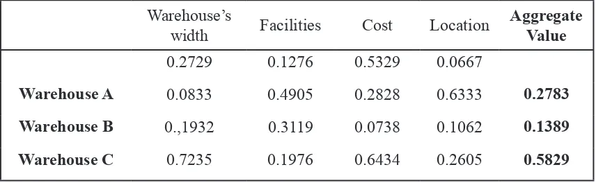
The determination of Alternative Ware-house based on the Highest Aggregate Score.

The last process in the calculation of Analytical Hierarchy Process (AHP) is to

calculate the aggregate score of each

alter-native warehouse which was obtained by

multiplying the priority score of each

alter-native on all criteria with a priority score of each criterion. The alternative warehouse that has the highest aggregate value is chosen as a reference in decision-making. Table 12 shows the aggregate scoring.

Conclusion

Warehouse C was selected as the

storage of finished good at PT. Frisian Flag

(8)

Soebagio. 1995. Manajemen Logistik.

(9)

n 1 2 3 4 5 6 7 8 9 10

RI 0 0 0,58 0,90 1,12 1,24 1,32 1,41 1,45 1,49

Focus Warehouse’s width Facilities Cost Location

4 digit

decimal

4 digit

decimal

4 digit

decimal

4 digit

decimal Warehouse’s

width

1 1.0000 3 3.0000 1/3 0.3333 5 5.0000

Facilities 1/3* 0.3333 1 1.0000 1/5 0.2000 3 3.0000

Cost 3* 3.0000 5* 5.0000 1 1.0000 5 5.0000

Location 1/5* 0.2000 1/3* 0.3333 1/5* 0.2000 1 1.0000

Total 4.5333 9.3333 1.7333 14.000

Focus Warehouse’s

width Facilities Cost Location

Priority Score

Warehouse’s width

0.2206 0.3214 0.1923 0.3571 0.2729

Facilities 0.0735 0.1072 0.1154 0.2144 0.1276

Cost 0.6618 0.5357 0.5769 0.3571 0.5329

Location 0.0441 0.0357 0.1154 0.0714 0.0666

Total 1.0000 1.0000 1.0000 1.0000 1.0000

Appendices

Tabel. 1 Random Index (RI) Score

Table 2 Pairwise Comparison Matrix of Warehouse Selection Criteria

Table 3 Normalized Matrix Source: Sri Mulyono (2002)

Source: Processed interview result * = reverse score (axioms reciprocal)

(10)

Warehouse’s

width criterion Warehouse A Warehouse B Warehouse C

4 digit decimal 4 digit decimal 4 digit deci

-mal

Warehouse A 1 1.0000 1/3 0.3333 1/7 0.1429

Warehouse B 3* 3.0000 1 1,0000 1/5 0.2000

Warehouse C 7* 7.0000 5* 5.0000 1 1.0000

Total 11.0000 6.3333 1.3429

Table 4 Warehouse’s width Pairwise Comparison Matrix

Source: Processed Interview result

* = reverse score (axioms reciprocal)

Warehouse’s

width criterion Warehouse A Warehouse B Warehouse C Priority Score

Warehouse A 0.0909 0.0526 0.1064 0.0833

Warehouse B 0.2727 0.1579 0.1489 0.1932

Warehouse C 0.6364 0.7895 0.7447 0.7235

Total 1.0000 1.0000 1.0000 1.0000

Warehouse’s

4 digit deci -mal

4 digit decimal 4 digit deci -mal

Warehouse A 1 1.0000 2 2.0000 2 2.0000

Warehouse B 1/2* 0.5000 1 1.0000 2 2.0000

Warehouse C 1/2* 0.5000 1/2* 0.5000 1 1.0000

Total 2.0000 3.5000 5.0000

Table 5 Normalized Matrix

Table 6 Facilities Pairwise Comparison Matrix Source: Processed Interview result

(11)

Warehouse’s

4 digit deci -mal

4 digit decimal 4 digit decimal

Warehouse A 1 1.0000 5 5.0000 1/3 0.3333

Warehouse B 1/5* 0.2000 1 1.0000 1/7 0.1429

Warehouse C 3* 3.0000 7* 7.0000 1 1.0000

Total 4.2000 13.0000 1.4762

Cost Criterion Warehouse A Warehouse B Warehouse C Priority Score

Warehouse A 0.2381 0.3846 0.2258 0.2828

Warehouse B 0.0476 0.0769 0.0968 0.0738

Warehouse C 0.7143 0.5385 0.6774 0.6434

Total 1.0000 1.0000 1.0000 1.0000

Table 8 Cost Pairwise Comparison Matrix

Table 9 Normalized Matrix Source: Processed Interview result

Facilities Criterion Warehouse A Warehouse B Warehouse C Priority Score

Warehouse A 0.5000 0.5714 0.4000 0.4905

Warehouse B 0.2500 0.2857 0.4000 0.3119

Warehouse C 0.2500 0.1429 0.2000 0.1976

Total 1.0000 1.0000 1.0000 1.0000

Table 7 Matriks Normalized

(12)

Warehouse’s

4 digit deci -mal

4 digit decimal 4 digit decimal

Warehouse A 1 1.0000 5 5.0000 3 3.0000

Warehouse B 1/5* 0.2000 1 1.0000 1/3 0.3333

Warehouse C 1/3* 0.3333 3* 3.0000 1 1.0000

Total 1.5333 9.0000 4.3333

Location Criterion Warehouse A Warehouse B Warehouse C Priority Score

Warehouse A 0.6522 0.5556 0.6923 0.6333

Warehouse B 0.1304 0.1111 0.0769 0.1062

Warehouse C 0.2174 0.3333 0.2308 0.2605

Total 1.0000 1.0000 1.0000 1.0000

Warehouse’s

width Facilities Cost Location

Aggregate Value

0.2729 0.1276 0.5329 0.0667

Warehouse A 0.0833 0.4905 0.2828 0.6333 0.2783

Warehouse B 0.,1932 0.3119 0.0738 0.1062 0.1389

Warehouse C 0.7235 0.1976 0.6434 0.2605 0.5829

Table 10 Location Pairwise Comparison Matrix

Table 11 Normalized Matrix

Table 22 Final Scoring of Each Alternative Source: Processed Interview result