Effect of Remediating MCAR
Data to Least Square Estimates
(LSE) of Non-Normal Data
MIRALUNA L. HERRERA
Missing Data Analysis
(Hair, et.al., 2007)
•
What is missing data?
•
What is the impact of missing data?
•
How to identify missing data?
–
Nature of missing data process
–
Extent of missingness
–
Randomness of missing data
process
–
Method of remediating missing
Objectives
•
To report the nature of missingness of the
samples with varying sample size in terms of:
–
p
-value deviation of sample sizes from the
MCAR missingness of the simulated data,
and
–
rate of missingness across varying sample
Objectives
•
To compare the methods in remediating missing
data in terms of the bias of regression coefficient
and standard error across varying sample size
- compare correlated normal data, & correlated
non-normal data
- compare uncorrelated and correlated non-normal
data
The Data
•
Work of Burdeos and Herrera (2011)
•
629 dengue incidence recorded in the Butuan
Medical Centre from June 2000 to July 2010
•
Variables – age of patient & number of days
confined in the hospital
•
Simulated data
n
=10, 20, 30, 50, 100 with
100 runs per
n
using
R
Methodology
Generating 20% MCAR
Randomization of
missing values
Little MCAR Test
Generating 20% MCAR
Randomization of
missing values
Little MCAR Test
Simulating MCAR 100 data
Remediating Missing Values
Data Processing in SPSS 15.0
Mean Substitution
Expectation Maximization
Multiple Imputations
Remediating Missing Values
Data Processing in SPSS 15.0
- correlated/uncorrelated variables
Computing
b
& SE
(in SPSS 15.0)
- correlated/uncorrelated variables
Computing % of
bias
(in MSExcel)
Computing % of
Data Processing in R-2.10.1-win32
Data EntryNote: Put NA for the missing values in the data set so that R executes the command.
> age<-scan() (Enter, then paste the copied one-column data from spreadsheet.) > days<-scan() (Enter, then paste the copied one-column data from spreadsheet.) > mat<-matrix(nrow=629, ncol=2)
> mat[ ,1]<-age > mat[ ,2]<-days > mat
Simulating 100 runs of n paired data (n=10, 20, 30, 50,100)
> # number of simulation nsim<-100
> # number of values per simulation
> nval<-n (In an actual simulation set specific value of n) mat2<-matrix(ncol=2*nsim, nrow=nval)
> for (i in 2*(1:nsim)){ temp<-c(1:nrow(mat)); c<-sample(temp, nval); mat2[ ,i-1]<- mat[c,1]; mat2[ ,i]<-mat[c,2]}
> mat2
Importing Data from R to Excel
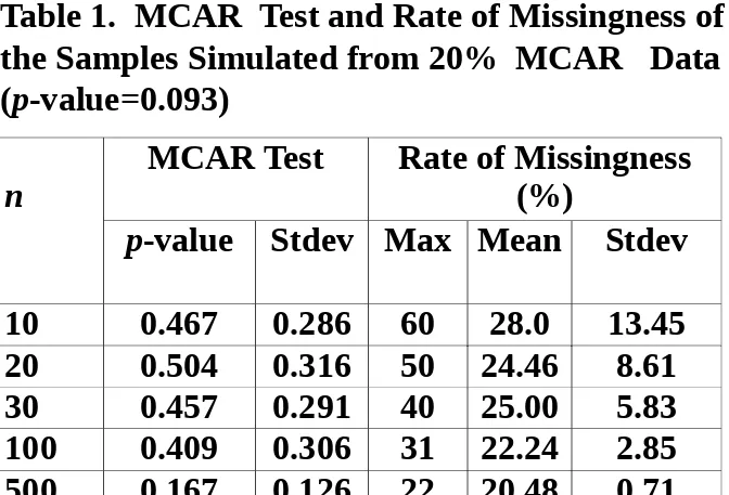
n
MCAR Test
Rate of Missingness
(%)
p
-value Stdev Max Mean
Stdev
10
0.467
0.286
60
28.0
13.45
20
0.504
0.316
50
24.46
8.61
30
0.457
0.291
40
25.00
5.83
100
0.409
0.306
31
22.24
2.85
500
0.167
0.126
22
20.48
0.71
Table 1. MCAR Test and Rate of Missingness of
the Samples Simulated from 20% MCAR Data
(
p
-value=0.093)
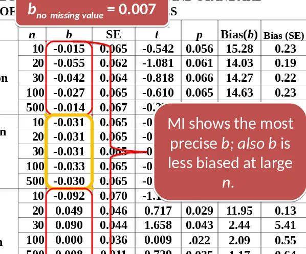
Method n b SE t p Bias(b) Bias (SE)
Mean
Substitution (MS)
10 -0.015 0.065 -0.542 0.056 15.28 0.23
20 -0.055 0.062 -1.081 0.061 14.03 0.19
30 -0.042 0.064 -0.818 0.066 14.27 0.22
100 -0.027 0.065 -0.610 0.065 14.63 0.23
500 -0.014 0.067 -0.379 0.062 15.43 0.26
Expectation
maximi-zation (EM)
10 -0.031 0.065 -0.686 0.062 14.73 0.23
20 -0.031 0.065 -0.686 0.062 14.73 0.23
30 -0.031 0.065 -0.686 0.062 14.73 0.23
100 -0.033 0.065 -0.707 0.063 14.65 0.23
500 -0.030 0.065 -0.653 0.063 14.74 0.23
Multiple Imputation (MI)
10 -0.092 0.070 -1.195 0.040 19.12 0.36
20 0.049 0.046 0.717 0.029 11.95 0.13
30 0.090 0.044 1.658 0.043 2.44 5.41
100 0.000 0.036 0.009 .022 2.09 0.55
500 0.008 0.011 0.729 0.035 1.17 0.64
Table 2. REGRESSION COEFFICIENTS AND STANDARD ERRORS OF CORRELATED VARIABLES
MI shows the most
precise b; also b is
less biased at large
n.
MI shows the most
precise
b; also b
is
less biased at large
n.
b
no missing value= 0.007
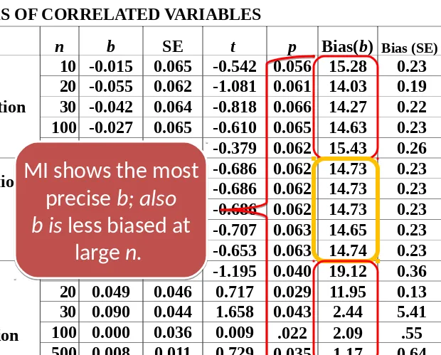
Method n b SE t p Bias(b) Bias (SE)
Mean
Substitution (MS)
10 -0.015 0.065 -0.542 0.056 15.28 0.23
20 -0.055 0.062 -1.081 0.061 14.03 0.19
30 -0.042 0.064 -0.818 0.066 14.27 0.22
100 -0.027 0.065 -0.610 0.065 14.63 0.23
500 -0.014 0.067 -0.379 0.062 15.43 0.26
Expectation
maximi-zation (EM)
10 -0.031 0.065 -0.686 0.062 14.73 0.23
20 -0.031 0.065 -0.686 0.062 14.73 0.23
30 -0.031 0.065 -0.686 0.062 14.73 0.23
100 -0.033 0.065 -0.707 0.063 14.65 0.23
500 -0.030 0.065 -0.653 0.063 14.74 0.23
Multiple Imputation (MI)
10 -0.092 0.070 -1.195 0.040 19.12 0.36
20 0.049 0.046 0.717 0.029 11.95 0.13
30 0.090 0.044 1.658 0.043 2.44 5.41
100 0.000 0.036 0.009 .022 2.09 .55
500 0.008 0.011 0.729 0.035 1.17 0.64
Table 2. REGRESSION COEFFICIENTS AND STANDARD ERRORS OF CORRELATED VARIABLES
MI shows the most
precise b; also
b is less biased at
large n.
MI shows the most
precise
b; also
Method n b SE t p Bias(b) Bias (SE)
Mean
Substitution (MS)
10 -0.015 0.065 -0.542 0.056 15.28 0.23
20 -0.055 0.062 -1.081 0.061 14.03 0.19
30 -0.042 0.064 -0.818 0.066 14.27 0.22
100 -0.027 0.065 -0.610 0.065 14.63 0.23
500 -0.014 0.067 -0.379 0.062 15.43 0.26
Expectation
maximi-zation (EM)
10 -0.031 0.065 -0.686 0.062 14.73 0.23
20 -0.031 0.065 -0.686 0.062 14.73 0.23
30 -0.031 0.065 -0.686 0.062 14.73 0.23
100 -0.033 0.065 -0.707 0.063 14.65 0.23
500 -0.030 0.065 -0.653 0.063 14.74 0.23
Multiple Imputation (MI)
10 -0.092 0.070 -1.195 0.040 19.12 0.36
20 0.049 0.046 0.717 0.029 11.95 0.13
30 0.090 0.044 1.658 0.043 2.44 5.41
100 0.000 0.036 0.009 0.022 2.09 0.55
500 0.008 0.011 0.729 0.035 1.17 0.64
Table 2. REGRESSION COEFFICIENTS AND STANDARD ERRORS OF CORRELATED VARIABLES
MI shows
relatively
small SE.
Estimation of
SE decreases
at large n.
MI shows
relatively
small SE
.
Estimation of
SE
decreases
at large
n.
SE
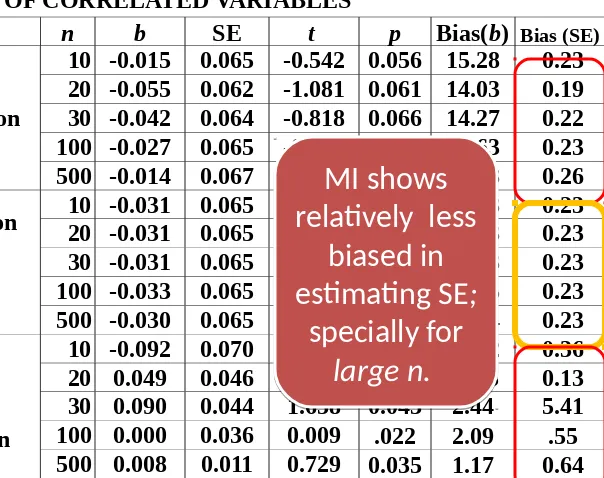
no missing value= 0.050
Method n b SE t p Bias(b) Bias (SE)
Mean
Substitution (MS)
10 -0.015 0.065 -0.542 0.056 15.28 0.23
20 -0.055 0.062 -1.081 0.061 14.03 0.19
30 -0.042 0.064 -0.818 0.066 14.27 0.22
100 -0.027 0.065 -0.610 0.065 14.63 0.23
500 -0.014 0.067 -0.379 0.062 15.43 0.26
Expectation
maximi-zation (EM)
10 -0.031 0.065 -0.686 0.062 14.73 0.23
20 -0.031 0.065 -0.686 0.062 14.73 0.23
30 -0.031 0.065 -0.686 0.062 14.73 0.23
100 -0.033 0.065 -0.707 0.063 14.65 0.23
500 -0.030 0.065 -0.653 0.063 14.74 0.23
Multiple Imputation (MI)
10 -0.092 0.070 -1.195 0.040 19.12 0.36
20 0.049 0.046 0.717 0.029 11.95 0.13
30 0.090 0.044 1.658 0.043 2.44 5.41
100 0.000 0.036 0.009 .022 2.09 .55
500 0.008 0.011 0.729 0.035 1.17 0.64
Table 2. REGRESSION COEFFICIENTS AND STANDARD ERRORS OF CORRELATED VARIABLES
MI shows
relatively less
biased in
estimating SE;
specially for
large n.
MI shows
relatively less
biased in
estimating SE
;
specially for
Method n b SE t p Bias(b) Bias (SE)
Mean
Substitution (MS)
10 -0.018 0.095 -0.104 0.506 7.97 0.70
20 -0.018 0.090 0.036 0.562 6.73 0.75
30 -0.015 0.089 0.054 0.567 6.48 0.74
100 -0.016 0.089 0.037 0.572 6.46 0.74
500 -0.018 0.089 0.019 0.576 6.39 0.75
Expectation maximization (EM)
10 -0.005 0.095 0.096 0.458 10.30 0.87
20 0.015 0.404 -1.320 0.544 29.08 5.55
30 0.039 0.139 0.711 0.481 14.61 1.70
100 -0.016 0.035 -0.390 0.503 4.25 0.48
500 0.000 0.011 0.018 0.538 0.99 0.55
Multiple Imputation (MI)
10 -0.018 0.095 -0.104 0.506 7.97 0.70
20 0.003 0.066 0.044 0.512 4.83 0.41
30 0.018 0.049 0.295 0.464 0.91 2.24
100 0.006 0.026 0.253 0.566 2.03 0.34
500 0.002 0.011 0.149 0.756 0.87 0.55
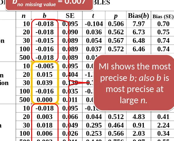
Table 3. REGRESSION COEFFICIENTS AND STANDARD ERRORS OF UNCORRELATED VARIABLES
MI shows the most
precise b; also b is
most precise at
large n.
MI shows the most
precise
b; also b
is
most precise at
large
n.
b
no missing value= 0.007
Method n b SE t p Bias(b) Bias (SE)
Mean
Substitution (MS)
10 -0.018 0.095 -0.104 0.506 7.97 0.70
20 -0.018 0.090 0.036 0.562 6.73 0.75
30 -0.015 0.089 0.054 0.567 6.48 0.74
100 -0.016 0.089 0.037 0.572 6.46 0.74
500 -0.018 0.089 0.019 0.576 6.39 0.75
Expectation
maximi-zation (EM)
10 -0.005 0.095 0.096 0.458 10.30 0.87
20 0.015 0.404 -1.320 0.544 29.08 5.55
30 0.039 0.139 0.711 0.481 14.61 1.70
100 -0.016 0.035 -0.390 0.503 4.25 0.48
500 0.000 0.011 0.018 0.538 0.99 0.55
Multiple Imputation (MI)
10 -0.018 0.095 -0.104 0.506 7.97 0.70
20 0.003 0.066 0.044 0.512 4.83 0.41
30 0.018 0.049 0.295 0.464 0.91 2.24
100 0.006 0.026 0.253 0.566 2.03 0.34
500 0.002 0.011 0.149 0.756 0.87 0.55
Table 3. REGRESSION COEFFICIENTS AND STANDARD ERRORS OF UNCORRELATED VARIABLES
MI shows the most
precise b; also
b is most precise at
large n.
MI shows the most
precise
b; also
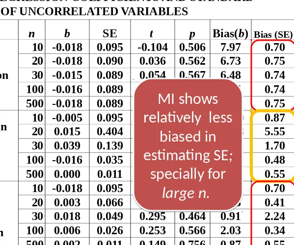
Method n b SE t p Bias(b) Bias (SE)
Mean
Substitution (MS)
10 -0.018 0.095 -0.104 0.506 7.97 0.70
20 -0.018 0.090 0.036 0.562 6.73 0.75
30 -0.015 0.089 0.054 0.567 6.48 0.74
100 -0.016 0.089 0.037 0.572 6.46 0.74
500 -0.018 0.089 0.019 0.576 6.39 0.75
Expectation
maximi-zation (EM)
10 -0.005 0.095 0.096 0.458 10.30 0.87
20 0.015 0.404 -1.320 0.544 29.08 5.55
30 0.039 0.139 0.711 0.481 14.61 1.70
100 -0.016 0.035 -0.390 0.503 4.25 0.48
500 0.000 0.011 0.018 0.538 0.99 0.55
Multiple Imputation (MI)
10 -0.018 0.095 -0.104 0.506 7.97 0.70
20 0.003 0.066 0.044 0.512 4.83 0.41
30 0.018 0.049 0.295 0.464 0.91 2.24
100 0.006 0.026 0.253 0.566 2.03 0.34
500 0.002 0.011 0.149 0.756 0.87 0.55
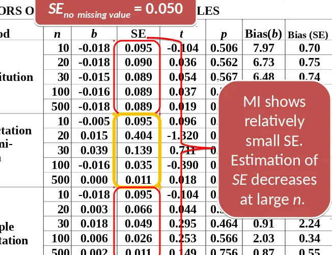
Table 3. REGRESSION COEFFICIENTS AND STANDARD ERRORS OF UNCORRELATED VARIABLES
MI shows
relatively
small SE.
Estimation of
SE decreases
at large n.
MI shows
relatively
small SE
.
Estimation of
SE
decreases
at large
n.
SE
no missing value= 0.050
Method n b SE t p Bias(b) Bias (SE)
Mean
Substitution (MS)
10 -0.018 0.095 -0.104 0.506 7.97 0.70
20 -0.018 0.090 0.036 0.562 6.73 0.75
30 -0.015 0.089 0.054 0.567 6.48 0.74
100 -0.016 0.089 0.037 0.572 6.46 0.74
500 -0.018 0.089 0.019 0.576 6.39 0.75
Expectation
maximi-zation (EM)
10 -0.005 0.095 0.096 0.458 10.30 0.87
20 0.015 0.404 -1.320 0.544 29.08 5.55
30 0.039 0.139 0.711 0.481 14.61 1.70
100 -0.016 0.035 -0.390 0.503 4.25 0.48
500 0.000 0.011 0.018 0.538 0.99 0.55
Multiple Imputation (MI)
10 -0.018 0.095 -0.104 0.506 7.97 0.70
20 0.003 0.066 0.044 0.512 4.83 0.41
30 0.018 0.049 0.295 0.464 0.91 2.24
100 0.006 0.026 0.253 0.566 2.03 0.34
500 0.002 0.011 0.149 0.756 0.87 0.55
Table 3. REGRESSION COEFFICIENTS AND STANDARD ERRORS OF UNCORRELATED VARIABLES
MI shows
relatively less
biased in
estimating SE;
specially for
large n.
MI shows
relatively less
biased in
estimating SE
;
specially for
Best Practices for Missing Data Management in Counseling Psychology Gabriel L. Schlomer, Sheri Bauman, and Noel A. Card, University of Arizona
Journal of Counseling Psychology 2010, Vol. 57, No. 1, 1–10
0022-© 2010 American Psychological Association, 0167/10/$12.00 DOI: 10.1037/a0018082
Best Practices for Missing Data Management in Counseling Psychology
Gabriel L. Schlomer, Sheri Bauman, and Noel A. Card, University of Arizona Journal of Counseling Psychology
2010, Vol. 57, No. 1, 1–10
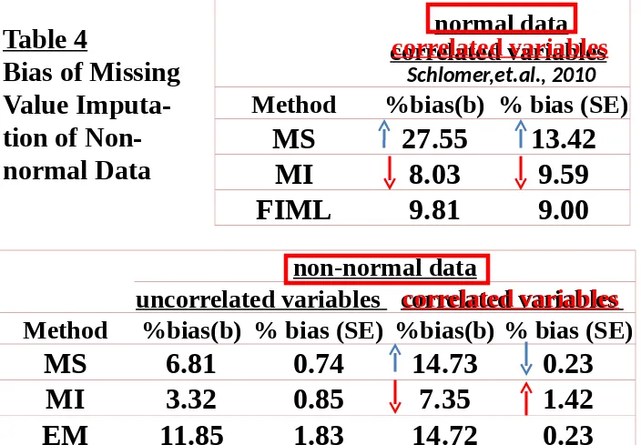
non-normal data
uncorrelated variables correlated variables
Method
%bias(b) % bias (SE) %bias(b) % bias (SE)
MS
6.81
0.74
14.73
0.23
MI
3.32
0.85
7.35
1.42
EM
11.85
1.83
14.72
0.23
normal data
correlated variables
Schlomer,et.al., 2010
Method
%bias(b) % bias (SE)
MS
27.55
13.42
MI
8.03
9.59
FIML
9.81
9.00
Table 4
Bias of Missing
Value
Imputa-tion of
Non-normal Data
correlated variables
non-normal data
uncorrelated variables correlated variables
Method
%bias(b) % bias (SE) %bias(b) % bias (SE)
MS
6.81
0.74
14.73
0.23
MI
3.32
0.85
7.35
1.42
EM
11.85
1.83
14.72
0.23
normal data
correlated variables
Schlomer,et.al., 2010