Identification of Macroeconomic Shocks:
Variations on the IS-LM Model
∗
Thomas J. Jordan
Swiss National Bank
Economic Studies Section
P.O. Box
CH–8022 Z¨
urich, Switzerland
E-mail: [email protected]
Carlos Lenz
Universit¨at Basel
WWZ
Petersgraben 51
CH–4003 Basel, Switzerland
E-mail: [email protected]
January 1999
Abstract
Applications of structural VARs to the IS-LM model reach different conclusions about the relative importance of demand and supply shocks for business cycle fluc-tuations. This paper analyzes why these discrepancies occur. It is shown that the results depend critically on the stationarity assumptions for certain variables. Be-cause the results of the unit root and cointegration tests are inconclusive, the results from structural VARs have to be interpreted with caution. It is crucial to check the sensitivity of the results with respect to the assumed order of integration of those variables which are on the borderline between I(1) and I(0).
JEL Classification: C32, E32
1. Introduction
The debate about which type of disturbances cause business cycle fluctuations stands tra-ditionally at the center of macroeconomic research. Since the seminal paper by Sims (1980), the basic tool to evaluate different shocks has been the vectorautoregression
(VAR). The critique by Cooley and LeRoy (1985) led to the development of the structural VAR approach pioneered by Bernanke (1986), Blanchard and Watson (1986), and Sims (1986).1
Recently, considerable interest has been devoted to structural VARs consisting of the variables which form the traditional IS-LM model. The restrictions needed to es-timate the structural VAR are taken from the long-run or short-run restrictions which are postulated by the aggregate supply/aggregate demand version of the textbook IS-LM
model.
There are two main motivations for this kind of analysis. One the one hand, the validity of the predictions of the IS-LM model can be tested empirically. This will answer
the question about the adequacy of the IS-LM model as a description of the economy.2
On the other hand, the relative impact of the structural shocks on the different variables
can be assessed. Of particular interest in this context is the following question: To what extent are output fluctuations at business cycle frequencies caused by either demand or supply shocks? This point is critical for a discussion of whether real business cycle theory or Keynesian macroeconomics is empirically more relevant.
There are five papers which can be regarded as applications of the IS-LM framework in a structural VAR analysis with postwar U.S. data: Gal´ı (1992), Keating (1992),
Bay-oumi and Eichengreen (1993)3
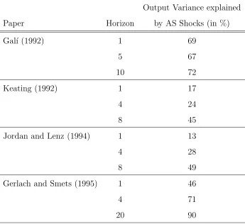
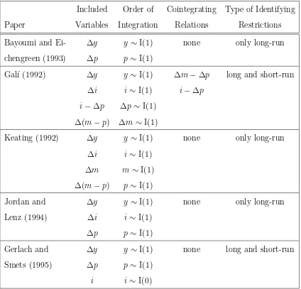
, Jordan and Lenz (1994), Gerlach and Smets (1995). The interesting point is that the results of these studies differ considerably, especially with respect to the importance of demand and supply shocks for output fluctuations. Table 1 summarizes the variance decompositions for output in the different studies.4
The following differences in the setup of the structural VARs can account for the
1
Structural VARs were originally identified by short-run restrictions. Blanchard and Quah (1989) and
Shapiro and Watson (1988) developed a method to identify shocks by long-run restrictions. Gal´ı (1992)
pioneered the simultaneous use of both types of restrictions.
2
See Gal´ı (1992) for a discussion why the empirical relevance of the IS-LM model remains of great
importance.
3
Two other papers by the same authors (Bayoumi and Eichengreen, 1994, 1995) use the same modeling
strategy. Unfortunately, none of their papers reports variance decompositions.
4
discrepancies among these papers: (1) the number of variables used to estimate the same
number of structural shocks, (2) the assumed order of integration of the variables and the assumed cointegrating relations, (3) the restrictions imposed to identify structural shocks, and (4) the used data sets (definition of the variables and sample periods). Table 2gives
an overview of the differences between the studies.
The number of variables included in all the analyzes varies between two and six. How-ever, the maximum number of variables entering a VAR is four, additional variables are sometimes analyzed by using linear combinations of the variables forming the estimated
system. The set of variables considered embraces output, the price level, real money, nominal money, as well as nominal and real interest rates. The number of variables
in-cluded in the VAR determines to what extent demand shocks have to be aggregated. The assumed order of integration of the variables differs, especially in the case of the inflation rate and the real interest rate. Most studies expect that the inflation rate is stationary,
only Gal´ı (1992) believes that it has a unit root. There is less consensus about the sta-tionarity of the real interest rate: half the papers which analyze this variable presuppose that it is stationary, the other half that it is integrated of order one. Depending on the
assumed order of integration of the individual variables, cointegration relations among them are implicit in the choice of variables used for the analysis. For instance, if the nominal interest rate and the inflation rate are assumed to be integrated of order one and
the real interest rate is taken to be stationary, then this implies that the nominal interest rate and the inflation rate are cointegrated. All the papers have the identification scheme for the aggregate supply shocks in common: Only these shocks have a long-run effect on
output. A variety of identification strategies are applied in order to identify the different demand shocks.
Even though part of the variation between the results of the studies can be attributed
to the use of different data sets it is still striking that empirical models based on the same philosophy come to very different conclusions. The purpose of this paper is therefore two-fold: First, by using the same set of data throughout our analysis, we investigate
why the above-mentioned papers reach different conclusions, especially with respect to the relative impact of demand and supply shocks on output over short horizons. Second, we try to assess which model specification is the correct one and try to show whether
demand shocks are in fact important for business cycle fluctuations.
is particularly true for the relative importance of demand and supply shocks. The
as-sumptions about the long-run properties of the variables also have an influence on the impulse responses but to a much lesser extent.It is interesting to note that the specific identification restrictions are less important for the variance decompositions. This is, of course, related to the fact that all authors use long-run neutrality of demand shocks to
identify aggregate supply shocks. However, the different strategies used to disentangle the different types of demand shocks have no dramatic consequences on their effects.
Fur-thermore, we find that a reduction in the number of variables implying the aggregation of demand shocks leaves the main results basically unchanged.Unit root and cointegration tests give no clear-cut answer about which model specification is the correct one.
There-fore, results from structural VARs have to be interpreted with caution, because the result may be sensitive to the assumed order of integration of those variables which are on the borderline between I(1) and I(0).
The remainder of this paper is organized as follows: Section 2presents the model and discusses its integration properties. In Section 3, we develop a method for identifying structural shocks in a VAR with both long-run and short-run restrictions. The empirical
results of five different specifications of the model are presented in Section 4, and Section 5 concludes.
2. A version of the IS-LM model
We start with the premise that real output, the nominal interest rate, nominal money, and the price level are the four variables that can be used to identify aggregate supply, money supply, money demand and spending shocks in a VAR model. Based on this assumption
we can ask two basic questions: 1. Which system of variables should be used? There are six variables to choose from, the four variables mentioned above plus some linear combinations like the real interest rate and real balances. In addition, each variable that
enters the system can be used in levels or in first differences (even second differences could be considered), which offers quite a wide range of options. 2. Which restrictions should be applied in order to identify the structural shocks? In the literature, a large variety of
approaches have been proposed to deal with this second question, but it is far from clear which of these solutions is optimal.
In order to answer these questions, we take both theoretical and empirical aspects
of integration should be in line with the structure of the model. Otherwise it becomes
an almost impossible task to apply the identifying restrictions suggested by the model. In addition, an empirical analysis is needed to establish the time series properties of the variables. In particular, this means that the empirical order of integration and possibly existing cointegrating relations among the variables should be tested for rather than
im-posed. The results of the unit root and cointegration tests can then be used to choose the correct specification of the model.
2.1. The model
In this section we present a log-linear version of the IS-LM model which is useful as a means of choosing the variables and their order of integration. The IS and LM equations
establish the usual equilibrium conditions in the goods and money markets
i−E∆p+1 = f +β1y (1)
m−p = d+β2y+β3i, (2)
wherei is the nominal interest rate,p is the price level, f are autonomous fiscal expendi-tures, y is output, m is money supply, and d is the autonomous part of money demand.
E and ∆ are the expectations and difference operators, respectively, and all variables, except the nominal interest rate, are in logs. The long-run aggregate supply curve is vertical. This means that long-run changes in output are governed by aggregate supply (uas) shocks
∆y = uas. (3)
In addition, we assume that the nominal money supply is either
∆m = β4∆y+β5∆i+β6umd+ums (4-a)
or
∆2
m = β4∆y+β5∆i+β6umd+ums, (4-b)
depending on the integration order of nominal money. Money supply depends therefore on all shocks in the model. Note that we consider equations (1) – (4) to be a long-run
Taking first differences and labeling changes in fiscal expenditures as IS-shocks (uis) and changes in the autonomous part of money demand as money demand shocks (umd), we can write the IS-LM model as follows:
∆(i−E∆p+1) = γ1∆y+uis (5)
where the choice of the price equation (8-a) or (8-b) depends on the integration order of
the money supply process. In order to derive equation (8-b), we impose a cointegrating relation between ∆m and ∆p.
If all variables on the right-hand side of these equations and the inflation rate are
stationary (which implies E∆2
p+1 = 0 or ∆p= ∆p+1), we can solve for the variables in
terms of the structural shocks:
This system represents the long-run effects of each structural shock and implies six
long-run neutrality restrictions: only aggregate supply shocks have a permanent effect on the level of output, monetary shocks have no permanent effect on the level of the real and the nominal interest rate, and money supply shocks have no permanent effect on the level of real balances.
If the inflation rate is non-stationary and money and prices are cointegrated, the model is
nominal interest rate and the inflation rate are cointegrated. In this case, the IS curve is
horizontal so that supply and fiscal shocks do not affect the real interest rate in the long run. In this case, only three exploitable long-run neutrality restrictions exist.
If the inflation rate is stationary, the model suggests six long-run neutrality restrictions which can be used to identify the structural shocks. If the inflation rate has a unit root,
the IS-LM model provides less than six long-run restrictions. In that case, short and long-run restrictions have to be combined in order to identify the structural VAR. The
short-run restrictions come from the less formal and more implicit assumption about the dynamics of the IS-LM model. For instance, Gal´ı (1992) assumes that output does not react contemporaneously to money demand and supply shocks. Other short-run
restrictions can be inferred from the assumptions about the money supply process.
2.2. Aggregation of demand shocks
As already mentioned above, some authors also use models consisting of only two or three variables and it is easy to see that this can be interpreted as an aggregation of demand
shocks. The money supply and money demand shocks can be aggregated to a money market shock (umm). By dropping the third line of equation (9), we get
This is the model used in Jordan and Lenz (1994) and comes quite close to the model
used by Gerlach and Smets (1995). Both papers use the nominal interest rate instead of the real interest rate. Since Gerlach and Smets (1995) assume the real interest rate to be stationary, however, they can only apply two long-run restrictions and therefore they
need a short-run restriction in order to separate monetary from fiscal shocks.
Going one step further, fiscal and monetary shocks can be aggregated to an aggregate demand shock. Eliminating the nominal interest rate from equation (11) yields
2.3. Variations on the IS-LM model
In order to find out where the discrepancies in the results of the different versions of the
IS-LM model come from, we estimate five empirical models:
Model 1 consists of the same VAR as in Gal´ı (1992), with a stationary real interest rate. However, we use a different set of short-run identifying restrictions, which allows us
to evaluate the influence of different identifying assumptions on the results. In the short run, prices do not react to money demand and money supply shocks. Furthermore, we presume that contemporaneous GNP does not enter the money supply rule.
Model 2 is the VAR formed by the variables of equation (9), where it is assumed that the inflation rate is stationary and the real interest rate has a unit root. In order to identify the structural shocks, we can rely on the long-run restrictions implied by the
model. The comparison of Model 1 and Model 2should shed some light on the impact of various systems on the results. Comparing Model 2to the long-run model of Keating (1992) should also give some insights about the discrepancies arising from using different
data sets.
Model 3 takes a unit root in both the inflation rate and the real interest rate. The VAR corresponds to equation (10). There are five long-run restrictions implied by the
model. Furthermore, we assume that the inflation rate does not react contemporaneously to money supply shocks. This exercise should give further insight into the effect of different systems on the results.
Model 4 corresponds to the three-variable system in equation (11), where we assume a stationary inflation rate and a non-stationary real interest rate. The shocks are identified
with long-run restrictions. This allows us to draw some conclusions about the use of different data sets and different types of restrictions as we compare the results to those in Jordan and Lenz (1994) and Gerlach and Smets (1995). In addition, we can assess the
effects of aggregating the money demand and supply shocks to a single money market shock.
results of Model 5 with those of Bayoumi and Eichengreen (1993) and those of Models 2
and 4 shows the effects of different data sets and the impact of the aggregation of all demand shocks to a single shock.
3. Identification of the structural shocks
The structural shocks of the IS-LM model can be identified by a combination of long-run and short-long-run identifying restrictions on the VAR representation of the variables in question. The idea of using both long-run and short-run restrictions simultaneously was
pioneered by Gal´ı (1992) and can be seen as a natural extension of earlier structural VAR approaches that proposed to use either only short-run or only long-run restrictions.
The implementation of the restrictions is a straightforward exercise, provided they
have a special kind of recursive structure as we can demonstrate for the general case. We start with a given vector of stationary variablesxt which is assumed to have a structural
vector moving average (VMA) representation
xt =A(L)ut,
where A(L) denotes a matrix polynomial in the lag-operator L and ut is a vector of
un-observable structural shocks. We assume that the structural shocks are mutually
uncor-related and normalize their variance to unity, i.e. E(utu′t) =I. Inversion of the structural
VMA representation yields the structural VAR representation
B(L)xt =ut,
where B(L) =A−1
(L). In order to identify the unobservable structural shocks contained in ut, a set of restrictions is placed on A(L) and B(L). This allows us to represent the
structural shocks as linear combinations of the disturbances of the reduced form system in xt.
We first estimate a reduced form VAR in xt
∆xt =D(L)∆xt−1+ǫt,
where ǫt is a vector of serially uncorrelated reduced form disturbances with covariance
matrix Ω. Inverting this VAR yields the Wold VMA representation
whereC0 equals the identity matrix. A comparison between the reduced form and
struc-tural VMAs immediately shows that the following relation must hold
A0ut =ǫt,
that is, onceA0 is known, the structural shocks can be computed from the reduced form
disturbances. In order to compute A0 we first note that
Ω = A0A
′
0,
which places n(n+ 1)/2restrictions on then2
different elements of A0. This means that
we need n(n−1)/2additional restrictions to identify A0. The method of Gal´ı (1992)
amounts to imposing restrictions on the immediate responses or the contemporaneous structural relations between the variables (given by A0 and B0 respectively) and on the
long-run responses to the structural shocks (given by A(1)). The additional restrictions are imposed on A0, either directly or via the relationships
A−1
0 =B0 and C(1)A0 =A(1).
Denoting the Cholesky decomposition of Ω by ˜Ω and an arbitrary orthonormal matrix by S, we can write:
Note that the knowledge of S is equivalent to the knowledge of A0 and, consequently,
that n(n−1)/2restrictions are needed to determine S. We show now that it is possible
to determine S explicitly if the restrictions have a ’triangular’ structure: Consider a (n−1)×n matrix Z which consists of the appropriate rows of ˜Ω, ( ˜Ω′)−1, and C(1) ˜Ω.
The ’triangular’ structure of the restrictions ensures thatZ can be ordered in such a way that, if multiplied by the first n−1 columns of S, the following holds
where Si denotes thei-th column of S. Using the equation above, the orthogonality of S
can be exploited to solve recursively for each of its columns:
MiSi =
In this section we carry out the estimation under the different setups discussed at the end of Section 2. We use the same data set as Gal´ı (1992). The sample period runs from 1955:I to 1987:III and the data includes the log of real GNP (y), the yield on three-month Treasury bills (i), the log of the Consumer Price Index (p), and the log of M1 (m). All data is from CITIBASE, except for measures of M1 previous to 1959 which are from the Federal Reserve Bulletin.
We then test for the order of integration of the individual variables and for possible cointegrating relations among some of the variables. These tests are critical for the fol-lowing reason: All variables included in the VAR have to be stationary to avoid spurious
regression problems. The estimated system is also misspecified if it includes first differ-ences of cointegrated variables. The empirical results of the unit root and cointegration tests are therefore a tool to discriminate among the different specifications in order to
find the correct model.
4.1. The Impact of Different Identifying Restrictions
We use the system proposed by Gal´ı (1992) to check whether different identification restrictions can lead to different impulse responses and variance decompositions. In
restrictions: MS and MD shocks do not affect the prices within the first quarter and
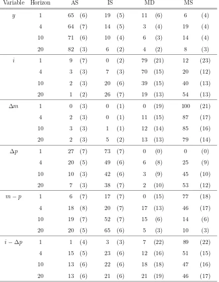
con-temporaneous GNP does not enter the money supply rule. The results are presented in Figure 1 and Table 5.
Considering the impulse responses, the only differences arising from using a new set of short-run identification restrictions are due to the impact of the MD shocks on ∆m, ∆p
andm−pin the short run. In our setup, nominal money growth first declines and becomes
positive only after 4 quarters. The inflation rate is first increasing and jumps below its
original level only after 8 quarters. Real balances therefore first decline and reach their old level after about 12quarters. All the other impulse responses look very similar to those reported to those in Gal´ı (1992). Concerning the variance decompositions, we find
that the relative importance of IS and MS shocks changes compared to Gal´ı’s results. In general MS shocks become more important for y, i, m, and ∆p; and less important for
m−pandi−∆p. The opposite is true for IS shocks. However, the impact of supply shocks
on all variables is very similar to Gal´ı (1992). Supply shocks are the dominant source of output fluctuations even in the very short run. We conclude that different identification restrictions do not lead to a change in the relative importance of demand and supply
shocks for output variations if the system remains unchanged.
With both possible identification schemes, the system proposed by Gal´ı leads to some implausible results. This is most evident in the version with the original set of restrictions.
IS shocks have a strong impact on the inflation rate in the long run, whereas MS supply shocks have a much smaller effect. IS shocks also have a strong impact on the long-run money growth. Although the IS shock has a positive impact on the inflation rate, it does
not influence the real interest rate. This is incompatible with conventional macroeconomic models.5
4.2. The Impact of Different Assumptions about the Order of Integration
We now concentrate on the effects of different assumptions about the order of integration
and estimate two new models: Model 2assumes that the inflation rate is stationary and that the real interest rate has a unit root; it consists of the variables ∆y, ∆(i−∆p), ∆p,
and ∆m−∆p. As discussed in Section 2, this model can be identified only by long-run
restrictions. Model 3 assumes that both the real interest rate and the inflation have a unit root; it consists of the variables ∆y, ∆(i−∆p), ∆2p, and ∆m−∆p and therefore
5
requires that ∆m and ∆p are cointegrated. The set of identification restrictions used in Model 3 is similar to the one used by Gal´ı (1992).
The results of Model 2are shown in Table 6 and Figure 2. Comparing the results to those of Model 1, the impulse responses are different for i, ∆p, and i−∆p. AS shocks
lower i and i−∆p in the long run, whereas IS shocks increase i and i−∆p. MS and
MD shocks have only a short-run impact on the interest rates. None of the shocks has a long-run impact on ∆pbecause of the assumed stationarity of ∆p. The impulse responses for output are similar to the system discussed above. All impulse responses of this model are exactly what we expect from the theoretical IS-LM model.
With respect to the variance decompositions, we observe a dramatic change. Demand
shocks, mainly IS and MS shocks, are now the dominant source of output fluctuations at business cycle frequencies. Consequently, different assumptions about the order of integration of the time series and the cointegration among the variables change the relative
importance of demand and supply shocks in the short run.
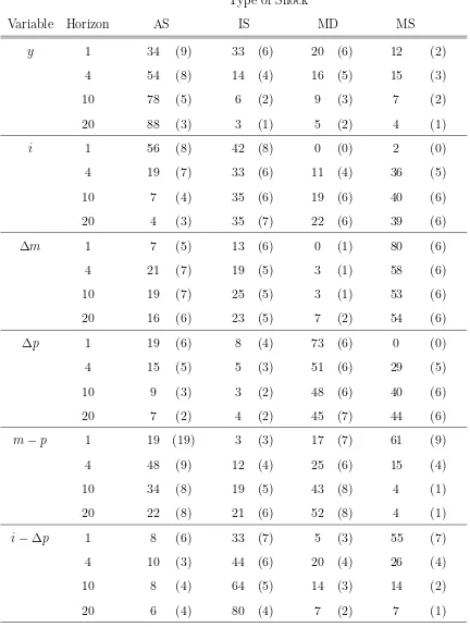
To further analyze the impact of a different integration assumptions on the results, we estimate Model 3. The results are in Table 7 and Figure 3. The impulse responses are
similar to those of Model 2. The main difference is the impulse response of the inflation rate which is not restricted to be zero in the long run. We find that changes in the inflation rate are mainly due to money demand and money supply shocks. It is interesting to note
that the contribution of demand shocks to the variance of real output lies between those of Models 1 and 2. In contrast to Model 1 demand shocks are important for output fluctuations in the short run, but not as important as in Model 2. All three demand
shocks contribute equally to output fluctuations, this implies that money demand shocks contribute more than in Model 2.
Keating (1992) uses a system which has the same assumptions about the order of
integration as our Model 2, but he uses the nominal interest rate instead of the real interest rate and money growth instead of inflation in his VAR setup. He also uses only long-run restrictions to identify the structural shocks. If we compare his results to those of
our Model 2, we find that they are very similar. However, in our Model 2, money supply shocks are generally more important than in the VAR used by Keating. Comparing the results of Keating (1992) to Model 1, we see again the dramatic change in the relative
importance of demand and supply shocks due to a different VAR system.
the assumed order of integration of the variables and, therefore, on whether the variables
enter the VAR in levels or in first differences. The results change completely for different integration assumptions. The use of different identification assumptions can also change the impulse responses of some variables, but the changes are less dramatic.
4.3. The Impact of Different Data Sets
Another question of some interest is whether the use of different data sets changes the results in any significant way if the same system is estimated. The comparison of either the results of Model 4 to those of Jordan and Lenz (1994) or those of Model 2to those of
Keating (1992) shows that the impulse responses are not very much influenced by different data sets. The variance decomposition shows that the relative impact of the different shocks changes. However, the relative importance of demand and supply shocks for output
fluctuations is approximately the same. Bayoumi and Eichengreen (1993) estimate a two-variable system, which can be compared to the system of equation (12). They do not present variance decompositions for their model. However, their impulse responses look
very similar to our results. We conclude that the use of different data sets does not affect the form of the impulse responses very much. However, the relative importance between the shocks can change. In the cases considered, the relative importance of demand and
supply shocks for output fluctuations remains the same for different data sets.
4.4. The Impact of Aggregation of Demand Shocks
An interesting aspect of the VAR analysis with IS-LM variables is the question whether the reduction of the four-variable VAR to a three and two-variable system changes the results
of the impulse responses and the variance decompositions. This point thus addresses the question whether the aggregation of structural demand shocks basically changes the importance of the demand shocks relative to the supply shocks.
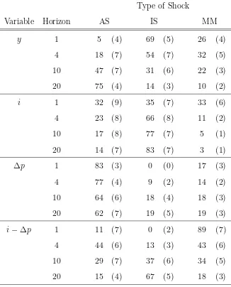
This question can be answered by looking at the results for Models 2, 4, and 5 which use only long-run restrictions to identify structural shocks. Model 4 aggregates money demand and supply shocks into a money market (MM) shock. The restrictions are that
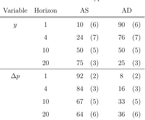
MM and IS shocks do not have long-run effects onyand MM shocks do not have long-run effects on i. In Model 5, all demand shocks are represented by a single aggregate demand (AD) shock which is assumed to leave output unaltered in the long run. Tables 8 and 9
If we compare the impact of the supply shocks on the output variance, we find a
relatively high correspondence between the three models. The relative importance of supply and demand shocks varies only slightly between the models. We therefore conclude that the reduction of the VAR or the aggregation of the shocks does not change the basic results of the relative importance between demand and supply shocks for output
fluctuations. The aggregation of shocks seems, in any case, less critical than the order of integration.
4.5. Unit Roots and Cointegration
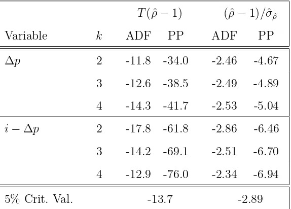
The order of integration for y, i, m, and m−p is undisputed. The results of our unit
root tests as well as those of other studies show that these variables are I(1).6
Therefore, we do not present the results of the unit root tests for these variables. The situation is
different for the inflation rate and the real interest rate. Table 3 shows the results of the Augmented-Dickey-Fuller and Phillips-Perron tests at different lag-lengths.7
The results of these unit root tests are mixed. For both variables, the Phillips-Perron tests reject the
null hypothesis of a unit root, whereas the Augmented-Dickey-Fuller tests point towards non-stationarity of the time series.
The studies of Keating (1992), Bayoumi and Eichengreen (1993), Gerlach and Smets
(1995), and Jordan and Lenz (1994) all assume the inflation rate to be stationary. The unit root tests presented in Gal´ı (1992) also indicate that the inflation rate is stationary. However, he concludes that the inflation rate must have a unit root because his tests
indicate that the real interest rate is stationary. This conclusion further implies cointe-gration between the nominal interest rate and the inflation rate. If the variables were not cointegrated, the real interest rate could not be stationary. A unit root in the inflation
rate also implies that ∆m is I(1) and cointegrated with ∆p if real money growth is to be stationary. This leads to an additional restriction for the order of integration of the variables included in the VAR.
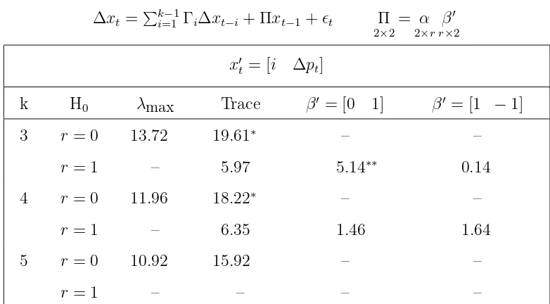
In order to shed some more light on this issue, we test for cointegration between iand ∆p as well as ∆m and ∆p by using the Johansen procedure. Table 4 summarizes the results of this exercise at different lag-lengths.
The tests show that the null hypothesis of no cointegration between i and ∆p is 6
An exception is the study by Gerlach and Smets (1995), whereiis assumed to be stationary.
7
The minimal lag-length for both the unit root and cointegration tests was chosen so that the residuals
never rejected if the maximum eigenvalue statistic is used. Considering the trace statistic
this hypothesis is rejected at the 10 percent level at lag-lengths 3 and 4, but we cannot reject the null of one cointegrating relation. However, this does not imply that the real interest rate is stationary. Given that i is I(1), the presence of only one unit root in the system consisting of i and ∆p can be due to either a stationary inflation rate or cointegration between i and ∆p, that is, a stationary real interest rate. In order to discriminate between these cases, we test whether the vectors [0 1] and [1 − 1] are
contained in the cointegrating space at those lag-lengths where a cointegrating relation between i and ∆p is found. The results are, again, unclear: At three lags, the presence of [0 1] in the cointegrating space is rejected, whereas the presence of [1 −1] cannot be
rejected. At four lags both vectors could be contained in the cointegrating space. To sum up, one can say that these results confirm the findings of the unit root tests: The data gives no clear answer to the question about the stationarity of ∆p and i−∆p.
Concerning the cointegration between ∆m and ∆p, the picture is not clear, either. The tests show that the null of no cointegration can be rejected at three lags in favor of one cointegrating relation. At four lags, only the maximum eigenvalue test rejects the
absence of cointegration; and at five lags, two unit roots seem to be present in the system formed by ∆m and ∆p. This contradicts the unit root tests where both real and nominal money appear to be stationary in first differences. At those lag-lengths where there seems
to be only one unit root in the system, we check whether it is due to the stationarity of ∆mor whether ∆mand ∆p are cointegrated. That is, we test whether the vectors [1 0] or [1 −1] are contained in the cointegrating space. The results of these tests show that
neither hypothesis can be rejected.
Given the evidence from the unit root and cointegration tests none of the models presented in Section 2can a priori be discarded. Furthermore, the exercise carried out in
this subsection does not provide the basis for a assessment of the models in accordance with their ability to fit the data. Therefore, the main conclusion we can draw from these tests is that one must be very cautious in interpreting the results from structural VARs.
5. Conclusions
We have presented a structural VAR analysis of the IS-LM model under a variety of identifying assumptions. The main contribution of this paper is to show that the relative importance of demand and supply shocks for output fluctuations depends critically on
the stationarity assumptions for certain variables. The responses of the variables to different shocks also depend to some extent on particular identifying restrictions, but those differences are less important. It is also shown that the aggregation of demand
shocks does not alter their relative importance with respect to supply shocks.
The obtained results show that in structural VAR analysis special care needs to be taken in determining the order of integration of the variables forming the estimated
sys-tem. This is particularly true in those cases where unit root tests do not yield clear results. With respect to the order of integration of the variables in the IS-LM model, the critical decision has to be made about the stationarity of both the real interest rate and
the inflation rate. If the real interest rate has a unit root and the inflation rate is station-ary, we see that demand shocks are very important for output fluctuations at business
cycle frequencies. If the real interest rate is stationary and the inflation rate has a unit root, then supply shocks are the dominant source of output fluctuations even in the short run. If both the real interest rate and the inflation rate have a unit root, the results are in-between the other two cases.
The evidence from the unit root and cointegration tests does not allow to favor one of the models over another. Therefore, one must be very cautious in interpreting the results
References
Bayoumi, T. and B. Eichengreen (1993) “Shocking aspects of european monetary unification.” In F. Torres and F. Giavazzi (eds.), Adjustment and Growth in the
Euro-pean Monetary Union. Cambridge University Press, Cambridge (UK).
Bayoumi, T. and B. Eichengreen(1994) “Macroeconomic adjustment under Bretton-Woods and the post Bretton-Bretton-Woods float: An impulse response analysis.” The
Eco-nomic Journal, 104:813–827.
Bayoumi, T. and B. Eichengreen(1995) “Is there a conflict between EC enlargement and European monetary unification?” Greek Economic Review.
Bernanke, B. S. (1986) “Alternative explanations of the money-income correlation.”
Carnegie-Rochester Conference Series on Public Policy, 25:49–100.
Blanchard, O. J. and D. Quah (1989) “The dynamic effects of aggregate demand and supply disturbances.” The American Economic Review, 79:655–673.
Blanchard, O. J. and M. Watson (1986) “Are business cycles all alike?” In R. Gor-don (ed.),The American Business Cycle, pp. 123–156. NBER and University of Chicago Press.
Cooley, T. F. and S. F. LeRoy (1985) “Atheoretical macroeconomics: A critique.”
Journal ofMonetary Economics, 16:283–308.
Gal´ı, J.(1992) “How well does the IS-LM model fit postwar U.S. data?” The Quarterly Journal ofEconomics, 107:709–738.
Gerlach, S. and F. Smets (1995) “The monetary transmission mechanism: Evidence from the G-7 countries.” Discussion Paper 1219, Center for European Policy Research.
Johansen, S. and K. Juselius(1990) “The full information maximum likelihood pro-cedure for inference on cointegration — with applications to the demand for money.”
Oxford Bulletin of Economics and Statistics, 52:169–210.
Keating, J. W. (1992) “Structural approaches to vector autoregressions.” Federal Re-serve Bank ofSt. Louis, Review, 74(5):37–57.
King, R. G. (1993) “Will the New Keynesian macroeconomics resurrect the IS-LM model?” Journal ofEconomic Perspectives, 7:67–82.
Osterwald-Lenum, M. (1992) “A note with quantiles of the asymptotic distribution of the maximum likelihood cointegration rank test statistics.” Oxford Bulletin of
Eco-nomics and Statistics, 54:461–472.
Runkle, D. E. (1987) “Vector autoregressions and reality.” Journal ofBusiness &
Economic Statistics, 5:437–442.
Shapiro, M. D. and M. W. Watson (1988) “Sources of business cycle fluctuations.” In S. Fischer (ed.), NBER Macroeconomics Annual 1988. The MIT Press, Cambridge
(Mass.) and London.
Sims, C. A. (1980) “Macroeconomics and reality.” Econometrica, 48:1–48.
Appendix: Tables and Figures
Table 1
Contribution of Supply Shocks to Fluctuations in U.S. GNP:
Results from four Studies
Output Variance explained
Paper Horizon by AS Shocks (in %)
Gal´ı (1992) 1 69
5 67
10 72
Keating (1992) 1 17
4 2 4
8 45
Jordan and Lenz (1994) 1 13
4 2 8
8 49
Gerlach and Smets (1995) 1 46
4 71
Table 2
VAR Setups in Different Studies
Included Order of Cointegrating Type of Identifying
Paper Variables Integration Relations Restrictions
Bayoumi and Ei- ∆y y∼I(1) none only long-run
chengreen (1993) ∆p p∼I(1)
Gal´ı (1992) ∆y y∼I(1) ∆m−∆p long and short-run
∆i i∼I(1) i−∆p
i−∆p ∆p∼ I(1)
∆(m−p) ∆m ∼I(1)
Keating (1992) ∆y y∼I(1) none only long-run
∆i i∼I(1)
∆m m∼I(1)
∆(m−p) p∼I(1)
Jordan and ∆y y∼I(1) none only long-run
Lenz (1994) ∆i i∼I(1)
∆p p∼I(1)
Gerlach and ∆y y∼I(1) none long and short-run
Smets (1995) ∆p p∼I(1)
Table 3
Unit Root Tests
T(ˆρ−1) (ˆρ−1)/σˆρˆ
Variable k ADF PP ADF PP
∆p 2-11.8 -34.0 -2.46 -4.67 3 -12.6 -38.5 -2.49 -4.89
4 -14.3 -41.7 -2.53 -5.04
i−∆p 2-17.8 -61.8 -2.86 -6.46
3 -14.2-69.1 -2.51 -6.70
4 -12.9 -76.0 -2.34 -6.94
5% Crit. Val. -13.7 -2.89
T(ˆρ−1) and (ˆρ−1)/σˆρˆdenote the modified bias and t-statistics
for the Augmented Dickey-Fuller (ADF) and the Phillips-Perron
(PP) tests respectively. The tests were carried out with
correc-tion for serial correlacorrec-tion atk lags. Both regressions include a
Table 4
Cointegration Tests
∆xt =k −1
i=1 Γi∆xt−i+ Πxt−1+ǫt Π
2×2
= α
2×r
β′ r×2
x′
t= [i ∆pt]
k H0 λmax Trace β
′
= [0 1] β′
= [1 −1]
3 r = 0 13.7219.61∗
– –
r = 1 – 5.97 5.14∗∗
0.14
4 r = 0 11.96 18.22∗
– –
r = 1 – 6.35 1.46 1.64
5 r = 0 10.9215.92 – –
r = 1 – – – –
x′
t= [∆mt ∆pt]
k H0 λmax Trace β
′
= [1 0] β′
= [1 −1]
3 r = 0 16.62∗∗
22.10∗∗∗
– –
r = 1 5.48 5.48 2.25 1.89 4 r = 0 14.16∗
18.51 – –
r = 1 4.35 – 2.19 1.78
5 r = 0 10.44 13.88 – –
r = 1 – – – –
∗,∗∗, and ∗∗ ∗denote significance at the 10, 5, and 1 percent levels, respectively. The columns labelled λmax and Trace contain the corresponding statistics for the
cointegration rank in the terminology of Johansen and Juselius (1990). Inference is
based on the critical values tabulated in Osterwald-Lenum (1992).
The last two columns contain the test statistics for the corresponding hypotheses
about the cointegration vectorsβ. In the present case they areχ2
1 distributed.
Table 5
Variance Decomposition: Model 1
Type of Shock
Variable Horizon AS IS MD MS
y 1 65 (6) 19 (5) 11 (6) 6 (4)
4 64 (7) 14 (5) 3 (4) 19 (4)
10 71 (6) 10 (4) 6 (3) 14 (4)
20 82 (3) 6 (2) 4 (2) 8 (3)
i 1 9 (7) 0 (2) 79 (21) 12 (23)
4 3 (3) 7 (3) 70 (15) 20 (12)
10 2(3) 20 (6) 39 (15) 40 (13)
20 1 (2) 26 (7) 19 (13) 54 (13)
∆m 1 0 (3) 0 (1) 0 (19) 100 (21)
4 2(3) 0 (1) 11 (15) 87 (17)
10 3 (3) 1 (1) 12(14) 85 (16)
20 2 (3) 5 (2) 13 (13) 79 (14)
∆p 1 27 (7) 73 (7) 0 (0) 0 (0)
4 20 (5) 49 (6) 6 (8) 25 (9)
10 10 (3) 42(6) 3 (9) 45 (10)
20 7 (3) 38 (7) 2 (10) 53 (12)
m−p 1 6 (7) 17 (7) 0 (15) 77 (18)
4 18 (8) 20 (7) 17 (13) 46 (17)
10 19 (7) 52(7) 15 (6) 14 (6)
20 20 (5) 65 (6) 5 (3) 10 (3)
i−∆p 1 1 (4) 3 (3) 7 (22) 89 (22)
4 15 (5) 23 (6) 12 (16) 51 (15)
10 13 (6) 22 (6) 18 (18) 47 (16)
20 13 (6) 21 (6) 21 (19) 46 (17)
Table 6
Variance Decomposition: Model 2
Type of Shock
Variable Horizon AS IS MD MS
y 1 6 (5) 66 (6) 1 (1) 27 (5)
4 12(7) 48 (8) 1 (1) 39 (6)
10 39 (7) 31 (7) 1 (1) 29 (4)
20 69 (5) 16 (4) 0 (0) 15 (2)
i 1 19 (8) 30 (7) 0 (1) 50 (8)
4 23 (7) 59 (7) 3 (1) 15 (2)
10 17 (7) 73 (7) 2(0) 8 (1)
20 15 (7) 79 (7) 1 (0) 5 (1)
∆m 1 4 (6) 1 (2) 67 (6) 28 (4)
4 11 (4) 8 (2) 52 (5) 30 (4)
10 11 (3) 11 (2) 50 (5) 28 (4)
20 13 (4) 10 (2) 48 (5) 29 (4)
∆p 1 77 (4) 0 (1) 15 (3) 7 (1)
4 73 (3) 5 (2) 13 (2) 8 (1)
10 60 (5) 12(3) 9 (2) 18 (3)
20 58 (5) 13 (4) 8 (1) 20 (3)
m−p 1 6 (6) 1 (3) 81 (6) 11 (2)
4 40 (8) 7 (3) 40 (6) 13 (2)
10 50 (7) 23 (5) 23 (4) 3 (1)
20 48 (8) 32 (6) 19 (3) 1 (0)
i−∆p 1 16 (10) 1 (3) 34 (7) 49 (7)
4 35 (7) 14 (4) 14 (3) 38 (5)
10 23 (6) 40 (5) 9 (2) 28 (4)
20 12 (3) 69 (4) 4 (1) 15 (3)
Table 7
Variance Decomposition: Model 3
Type of Shock
Variable Horizon AS IS MD MS
y 1 34 (9) 33 (6) 20 (6) 12 (2)
4 54 (8) 14 (4) 16 (5) 15 (3)
10 78 (5) 6 (2) 9 (3) 7 (2)
20 88 (3) 3 (1) 5 (2) 4 (1)
i 1 56 (8) 42(8) 0 (0) 2 (0)
4 19 (7) 33 (6) 11 (4) 36 (5)
10 7 (4) 35 (6) 19 (6) 40 (6)
20 4 (3) 35 (7) 22 (6) 39 (6)
∆m 1 7 (5) 13 (6) 0 (1) 80 (6)
4 21 (7) 19 (5) 3 (1) 58 (6)
10 19 (7) 25 (5) 3 (1) 53 (6)
20 16 (6) 23 (5) 7 (2) 54 (6)
∆p 1 19 (6) 8 (4) 73 (6) 0 (0)
4 15 (5) 5 (3) 51 (6) 29 (5)
10 9 (3) 3 (2) 48 (6) 40 (6)
20 7 (2) 4 (2) 45 (7) 44 (6)
m−p 1 19 (19) 3 (3) 17 (7) 61 (9)
4 48 (9) 12(4) 25 (6) 15 (4)
10 34 (8) 19 (5) 43 (8) 4 (1)
20 22 (8) 21 (6) 52 (8) 4 (1)
i−∆p 1 8 (6) 33 (7) 5 (3) 55 (7)
4 10 (3) 44 (6) 20 (4) 26 (4)
10 8 (4) 64 (5) 14 (3) 14 (2)
20 6 (4) 80 (4) 7 (2) 7 (1)
Table 8
Variance Decomposition: Model 4
Type of Shock
Variable Horizon AS IS MM
y 1 5 (4) 69 (5) 26 (4)
4 18 (7) 54 (7) 32(5)
10 47 (7) 31 (6) 22 (3)
20 75 (4) 14 (3) 10 (2)
i 1 32(9) 35 (7) 33 (6)
4 23 (8) 66 (8) 11 (2)
10 17 (8) 77 (7) 5 (1)
20 14 (7) 83 (7) 3 (1)
∆p 1 83 (3) 0 (0) 17 (3)
4 77 (4) 9 (2) 14 (2)
10 64 (6) 18 (4) 18 (3)
20 62 (7) 19 (5) 19 (3)
i−∆p 1 11 (7) 0 (2) 89 (7)
4 44 (6) 13 (3) 43 (6)
10 29 (7) 37 (6) 34 (5)
20 15 (4) 67 (5) 18 (3)
Table 9
Variance Decomposition: Model 5
Type of Shock
Variable Horizon AS AD
y 1 10 (6) 90 (6)
4 24 (7) 76 (7)
10 50 (5) 50 (5)
20 75 (3) 25 (3)
∆p 1 92 (2) 8 (2)
4 84 (3) 16 (3)
10 67 (5) 33 (5)
20 64 (6) 36 (6)
Figure 1
Model 1
Responses to AS-Shock Responses to IS-Shock
Figure 2
Model 2
Responses to AS-Shock Responses to IS-Shock
Figure 3
Model 3
Responses to AS-Shock Responses to IS-Shock
Figure 4
Model 4
Responses to AS-Shock Responses to IS-Shock
Responses to MM-Shock
Figure 5
Model 5