Linear and nonlinear programming (5)

Programming”

David G. Luenberger and Yinyu Ye

Contents

Preface

ix

List of Figures

xi

5

Interior-Point Algorithms

117

5.1

Introduction . . . .

117

5.2

The simplex method is not polynomial-time

∗

_{. . . .}

₁₂₀

5.3

The Ellipsoid Method . . . .

125

5.4

The Analytic Center . . . .

128

5.5

The Central Path . . . .

131

5.6

Solution Strategies . . . .

137

5.6.1

Primal-dual path-following

. . . .

139

5.6.2

Primal-dual potential function

. . . .

141

5.7

Termination and Initialization

∗

_{. . . .}

₁₄₄

5.8

Notes

. . . .

148

5.9

Exercises

. . . .

149

12 Penalty and Barrier Methods

153

12.9 Convex quadratic programming . . . .

153

12.10Semidefinite programming . . . .

154

12.11Notes

. . . .

158

12.12Exercises

. . . .

159

Bibliography

160

Index

409

Preface

List of Figures

5.1

Feasible region for Klee-Minty problem;

n

= 2. . . .

121

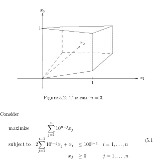
5.2

The case

n

= 3. . . .

122

5.3

Illustration of the minimal-volume ellipsoid containing a

half-ellipsoid. . . .

127

5.4

The central path as analytic centers in the dual feasible region.135

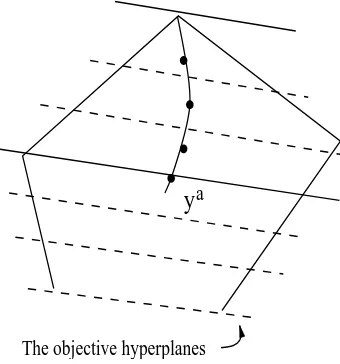
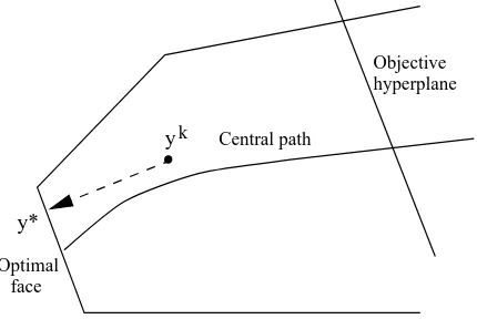
5.5

Illustration of the projection of an interior point onto the

optimal face.

. . . .

146

Chapter 5

Interior-Point Algorithms

5.1

Introduction

Linear programming (LP), plays a distinguished role in optimization theory.

In one sense it is a continuous optimization problem since the goal is to

minimize a linear objective function over a convex polyhedron. But it is

also a combinatorial problem involving selecting an extreme point among

a finite set of possible vertices, as seen in Chapters 3 and 4.

An optimal solution of a linear program always lies at a vertex of the

feasible region, which itself is a polyhedron. Unfortunately, the number of

vertices associated with a set of

n

inequalities in

m

variables can be

expo-nential in the dimension—up to

n!/m!(n

−

m)!. Except for small values of

m

and

n, this number is sufficiently large to prevent examining all possible

vertices when searching for an optimal vertex.

The simplex method examines optimal candidate vertices in an

intel-ligent fashion. As we know, it constructs a sequence of adjacent vertices

with improving values of the objective function. Thus, the method travels

along edges of the polyhedron until it hits an optimal vertex. Improved in

various way in the intervening four decades, the simplex method continues

to be the workhorse algorithm for solving linear programming problems.

Although it performs well in practice, the simplex method will examine

every vertex when applied to certain linear programs. Klee and Minty in

1972 gave such an example. These examples confirm that, in the worst

case, the simplex method uses a number of iterations that is exponential

in the size of the problem to find the optimal solution. As interest in

complexity theory grew, many researchers believed that a good algorithm

should be polynomial —that is, broadly speaking, the running time required

to compute the solution should be bounded above by a polynomial in the

size, or the total data length, of the problem. The simplex method is not

a polynomial algorithm.

1

In 1979, a new approach to linear programming, Khachiyan’s ellipsoid

method, received dramatic and widespread coverage in the international

press. Khachiyan proved that the ellipsoid method, developed during the

1970s by other mathematicians, is a polynomial algorithm for linear

pro-gramming under a certain computational model. It constructs a sequence

of shrinking ellipsoids with two properties: the current ellipsoid always

con-tains the optimal solution set, and each member of the sequence undergoes

a guaranteed reduction in volume, so that the solution set is squeezed more

tightly at each iteration.

Experience with the method, however, led to disappointment. It was

found that even with the best implementations the method was not even

close to being competitive with the simplex method.

Thus, after the

dust eventually settled, the prevalent view among linear programming

re-searchers was that Khachiyan had answered a major open question on the

polynomiality of solving linear programs, but the simplex method remained

the clear winner in practice.

This contradiction, the fact that an algorithm with the desirable

the-oretical property of polynomiality might nonetheless compare unfavorably

with the (worst-case exponential) simplex method, set the stage for

excit-ing new developments. It was no wonder, then, that the announcement by

Karmarkar in 1984 of a new polynomial time algorithm, an interior-point

method, with the potential to improve the practical effectiveness of the

simplex method made front-page news in major newspapers and magazines

throughout the world.

Interior-point algorithms are continuous iterative algorithms.

Computa-tional experience with sophisticated procedures suggests that the number

of necessary iterations grows very slowly with problem size. This

pro-vides the potential for improvements in computation effectiveness for

solv-ing large-scale linear programs. The goal of this chapter is to provide

some understanding on the complexity theories of linear programming and

polynomial-time interior-point algorithms.

A few words on complexity theory

5.1.

INTRODUCTION

₁₁₉

measuring the effectiveness of various algorithms (and thus, be able to

com-pare algorithms using these criteria), and to assess the inherent difficulty

of various problems.

The term

complexity

refers to the amount of resources required by a

computation. In this chapter we focus on a particular resource, namely,

computing time. In complexity theory, however, one is not interested in

the execution time of a program implemented in a particular programming

language, running on a particular computer over a particular input. This

involves too many contingent factors. Instead, one wishes to associate to

an algorithm more intrinsic measures of its time requirements.

Roughly speaking, to do so one needs to define:

•

a notion of

input size,

•

a set of

basic operations, and

•

a

cost

for each basic operation.

The last two allow one to associate a

cost of a computation. If

x

is any

input, the cost

C(x) of the computation with input

x

is the sum of the

costs of all the basic operations performed during this computation.

Let

A

be an algorithm and

In

be the set of all its inputs having size

n.

The

worst-case cost function

of

A

is the function

T

w

A

defined by

T

w

A

(n) = sup

x∈In

C(x).

If there is a probability structure on

In

it is possible to define the

average-case cost function

T

a

A

given by

T

a

A(n) = En(C(x)).

where En

is the expectation over

In. However, the average is usually more

difficult to find, and there is of course the issue of what probabilities to

assign.

the size of an element is usually taken to be 1 and consequently to have

unit size

per number.

Examples of the second are integer numbers which require a number

of bits approximately equal to the logarithm of their absolute value. This

(base 2) logarithm is usually referred to as the

bit size

of the integer. Similar

ideas apply for rational numbers.

Let

A

be some kind of data and

x

_{= (x}

₁

, . . . , xn

)

∈

A

n

. If

A

is of

the first kind above then we define size(

x

_{) =}

_{n. Otherwise, we define}

size(

x

_{) =}

P

n

_i

=1

bit-size(xi

).

The cost of operating on two unit-size numbers is taken to be 1 and is

called

unit cost. In the bit-size case, the cost of operating on two numbers

is the product of their bit-sizes (for multiplications and divisions) or its

maximum (for additions, subtractions, and comparisons).

The consideration of integer or rational data with their associated bit

size and bit cost for the arithmetic operations is usually referred to as the

Turing model of computation. The consideration of idealized reals with unit

size and unit cost is today referred as the

real number arithmetic model.

When comparing algorithms, one should make clear which model of

com-putation is used to derive complexity bounds.

A basic concept related to both models of computation is that of

poly-nomial time. An algorithm

A

is said to be a polynomial time algorithm if

T

w

A

is bounded above by a polynomial. A problem can be solved in

polyno-mial time if there is a polynopolyno-mial time algorithm solving the problem. The

notion of

average polynomial time

is defined similarly, replacing

T

w

A

by

T

a

A.

The notion of polynomial time is usually taken as the formalization of

efficiency and it is the ground upon which complexity theory is built.

5.2

The simplex method is not

polynomial-time

∗

When the simplex method is used to solve a linear program in standard

form with the coefficient matrix

A

∈

R

m×n

,

b

∈

R

m

and

c

∈

R

n

, the

number of iterations to solve the problem starting from a basic feasible

solution is typically a small multiple of

m: usually between 2m

and 3m.

In fact, Dantzig observed that for problems with

m

≤

50 and

n

≤

200 the

number of iterations is ordinarily less than 1.5m.

5.2.

THE SIMPLEX METHOD IS NOT POLYNOMIAL-TIME

∗

₁₂₁

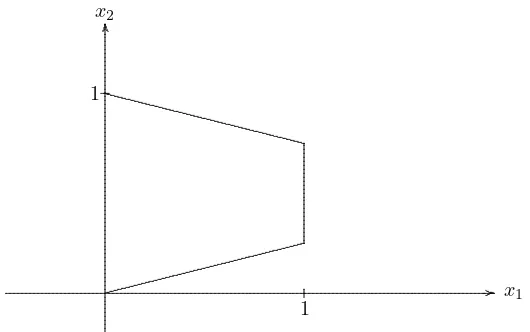
Figure 5.1: Feasible region for Klee-Minty problem;n

= 2.

paper that exhibited a class of linear programs each of which requires an

exponential number of iterations when solved by the conventional simplex

method.

As originally stated, the Klee–Minty problems are not in standard form;

they are expressed in terms of 2n

linear inequalities in

n

variables. Their

feasible regions are perturbations of the

unit cube

_in

_{n-space; that is,}

[0,

1]

n

₌

_{x

_{: 0}

_≤

_xj

_≤

_1,

_j

_{= 1, . . . , n}.}

One way to express a problem in this class is

maximize

xn

subject to

x

₁

≥

0

x

1

≤

1

xj

≥

εxj

−1

j

= 2, . . . , n

xj

≤

1

−

εxj

−1

j

= 2, . . . , n

where 0

< ε <

1/2.

This presentation of the problem emphasizes the idea

that the feasible region of the problem is a perturbation of the

n-cube.

In the case of

n

= 2 and

ε

= 1/4, the feasible region of the linear

program above looks like that of Figure 5.1

.

subject to

2

i

−

1

The problem above is easily cast as a linear program in standard form.

Example 5.1

Suppose we want to solve the linear program

maximize

100x

1

+ 10x

2

+

x

3

subject to

x

1

≤

1

20x

1

+

x

2

≤

100

200x

1

+ 20x

2

+

x

3

≤

10,

000

5.2.

THE SIMPLEX METHOD IS NOT POLYNOMIAL-TIME

∗

₁₂₃

T

0

Variable

x1

x2

x3

x4

x5

x6

b

4

1

0

0

1

0

0

1

5

20

1

0

0

1

0

100

6

200

20

1

0

0

1

10,000

c

T

₁₀₀

₁₀

₁

₀

₀

₀

₀

•

•

•

The bullets below the tableau indicate the columns that are basic.

Note that we are maximizing, so the goal is to find a feasible basis that

prices out

nonpositive

. In the objective function, the nonbasic variables

x1, x2,

and

x3

have coefficients 100, 10, and 1, respectively. Using the

greedy rule

2

for selecting the incoming variable (see Section 3.8, Step 2

of the revised simplex method), we start making

x1

positive and find (by

the minimum ratio test) that

x4

becomes nonbasic. After pivoting on the

element in row 1 and column 1, we obtain a sequence of tables:

T

1

Variable

x1

x2

x3

x4

x5

x6

b

1

1

0

0

1

0

0

1

5

0

1

0

–20

1

0

80

6

0

20

1

–200

0

1

9,800

r

T

₀

₁₀

₁

_–100

₀

₀

_–100

•

•

•

T

2

Variable

x1

x2

x3

x4

x5

x6

b

1

1

0

0

1

0

0

1

2

0

1

0

–20

1

0

80

6

0

0

1

200

–20

1

8,200

r

T

₀

₀

₁

₁₀₀

_–10

₀

_–900

•

•

•

T

3

Variable

x1

x2

x3

x4

x5

x6

b

4

1

0

0

1

0

0

1

2

20

1

0

0

1

0

100

6

–200

0

1

0

–20

1

8,000

r

T

_–100

₀

₁

₀

_–10

₀

_–1,000

•

•

•

T

4

Variable

x1

x2

x3

x4

x5

x6

b

4

1

0

0

1

0

0

1

2

20

1

0

0

1

0

100

3

–200

0

1

0

–20

1

8,000

r

T

₁₀₀

₀

₀

₀

₁₀

_–1

_–9,000

•

•

•

T

5

Variable

x1

x2

x3

x4

x5

x6

b

1

1

0

0

1

0

0

1

2

0

1

0

–20

1

0

80

3

0

0

1

200

–20

1

8,200

r

T

0

0

0

–100

10

–1

–9,100

•

•

•

T

6

Variable

x1

x2

x3

x4

x5

x6

b

1

1

0

0

1

0

0

1

5

0

1

0

–20

1

0

80

3

0

20

1

–200

0

1

9,800

r

T

0

–10

0

100

0

–1

–9,900

•

•

•

T

7

Variable

x1

x2

x3

x4

x5

x6

b

4

1

0

0

1

0

0

1

5

20

1

0

0

1

0

100

3

200

20

1

0

0

1

10,000

r

T

–100

–10

0

0

0

–1

–10,000

•

•

•

From T

7

we see that the corresponding basic feasible solution

(x1, x2, x3, x4, x5, x6) = (0,

0,

10

4

,

1,

10

2

,

0)

is optimal and that the objective function value is 10

,

000

.

Along the way,

we made 2

3

−

1 = 7 pivot steps. The objective function strictly increased

with each change of basis.

We see that the instance of the linear program (5.1) with

n

= 3 leads to

2

3

−

1 pivot steps when the greedy rule is used to select the pivot column.

The general problem of the class (5.1) takes 2

n

−

1 pivot steps. To get

an idea of how bad this can be, consider the case where

n

= 50. Now

2

50

−

1

≈

10

15

.

In a year with 365 days, there are approximately 3

_×

10

7

seconds. If a computer ran continuously performing a hundred thousand

iterations of the simplex algorithm per second, it would take approximately

10

15

3

×

10

5

×

10

8

≈

33 years

to solve the problem using the greedy pivot selection rule

3

.

3

5.3.

THE ELLIPSOID METHOD

₁₂₅

5.3

The Ellipsoid Method

The basic ideas of the ellipsoid method stem from research done in the

nineteen sixties and seventies mainly in the Soviet Union (as it was then

called) by others who preceded Khachiyan. The idea in a nutshell is to

enclose the region of interest in each member of a sequence of ever smaller

ellipsoids.

The significant contribution of Khachiyan was to demonstrate in two

papers—published in 1979 and 1980—that under certain assumptions, the

ellipsoid method constitutes a polynomially bounded algorithm for linear

programming.

The method discussed here is really aimed at finding a point of a

poly-hedral set Ω given by a system of linear inequalities.

Ω =

{

y

∈

R

m

_:

_y

T

_a

j

≤

cj,

j

= 1, . . . n}

Finding a point of Ω can be thought of as being equivalent to solving a

linear programming problem.

Two important assumptions are made regarding this problem:

(A1) There is a vector

y0

∈

R

m

_{and a scalar}

_{R >}

_{0 such that the closed}

ball

S(y0

, R) with center

y0

and radius

R, that is

{

y

∈

R

m

_:

_|

_y

₋

_y0

_{| ≤}

_R},

contains Ω.

(A2) There is a known scalar

r >

0 such that if Ω is nonempty, then it

contains a ball of the form

S(y

∗

_{, r) with center at}

_y

∗

_{and radius}

r. (This assumption implies that if Ω is nonempty, then it has a

nonempty interior and its volume is at least vol(S(0, r)))

4

.

Definition 5.1

An

Ellipsoid

in

R

m

_{is a set of the form}

E

=

{y

∈

R

m

: (y

−

z)

T

_Q(y

₋

_z)

_≤

_1}

where

z

∈

R

m

_{is a given point (called the}

_{center) and}

_Q

_{is a positive definite}

matrix (see Section A.4 of Appendix A) of dimension

m. This ellipsoid is

denoted ell(z,

Q).

The unit sphere

S(0,

1) centered at the origin

0

is a special ellipsoid

with

Q

=

I

, the identity matrix.

The axes of a general ellipsoid are the eigenvectors of

Q

and the lengths

of the axes are

λ

−

1

/

2

1

, λ

−

1

/

2

2

, . . . , λ

−

1

/

2

m

, where the

λi’s are the corresponding

eigenvalues. It is easily seen that the volume of an ellipsoid is

vol(E) = vol(S(0,

1))Π

m

i

=1

λ

−

1

/

2

i

= vol(S(0,

1))det(Q

−

1

/

2

_).

Cutting plane and new containing ellipsoid

In the ellipsoid method, a series of ellipsoids

Ek

are defined, with centers

y

k

and with the defining

Q

=

B

−

k

1

,

where

B

k

is symmetric and positive

definite.

At each iteration of the algorithm, we will have Ω

⊂

Ek. It is then

possible to check whether

y

k

∈

Ω.

If so, we have found an element of Ω as

required. If not, there is at least one constraint that is violated. Suppose

a

T

_j

y

k

> cj.

Then

Ω

⊂

1

2

Ek

:=

{

y

∈

Ek

:

a

T

j

y

≤

a

T

j

y

k}

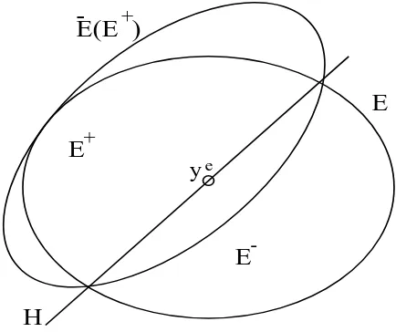
This set is half of the ellipsoid, obtained by cutting the ellipsoid in half

through its center.

The successor ellipsoid

Ek

+1

will be the minimal-volume ellipsoid

con-taining

1

₂

Ek

. It is constructed as follows. Define

τ

=

1

m

+ 1

,

δ

=

m

2

m

2

₋

₁

,

σ

= 2τ.

Then put

y

k

+1

=

y

k

−

τ

(a

T

j

B

k

a

j

)

1

/

2

B

k

a

j

B

k

+1

=

δ

Ã

B

k

−

σ

Bkaja

T

_j

Bk

a

T

_j

B

k

a

j

!

(5.2)

.

Theorem 5.1

The ellipsoid

Ek

+1

= ell(yk

+1

,

B

−

_k

₊₁

1

)

defined as above is

the ellipsoid of least volume containing

1

₂

Ek

. Moreover,

vol(Ek

+1

)

vol(Ek

)

=

µ

_m

2

m

2

₋

₁

¶

(

m

−

1)

/

2

_m

m

+ 1

<

exp

µ

−

1

2(m

+ 1)

¶

5.3.

THE ELLIPSOID METHOD

₁₂₇

E

+

-E

E

H

y

e

E(E )

-

+

Figure 5.3: Illustration of the minimal-volume ellipsoid containing a

half-ellipsoid.

Proof.

_{We shall not prove the statement about the new ellipsoid being}

of least volume, since that is not necessary for the results that follow. To

prove the remainder of the statement, we have

vol(

E

_k

₊₁

₎

vol(

E

_k

₎

=

det(B

1

_k

/

₊₁

2

)

det(B

1

_k

/

2

)

For simplicity, by a change of coordinates, we may take

B

k

=

I

.

Then

B

k

+1

has

m

−

1 eigenvalues equal to

δ

=

m

2

m

2

₋

1

and one eigenvalue equal

to

δ

−

2

δτ

₌

m

2

m

2

₋

1

(1

−

2

m

+1

) = (

m

m

+1

)

2

.

The reduction in volume is the

product of the square roots of these, giving the equality in the theorem.

Then using (1 +

x

₎

p

_≤

_e

xp

_{, we have}

µ

_m

2

m

2

₋

₁

¶

(

m

−

1)

/

2

_m

m

_{+ 1}

=

µ

1 +

1

m

2

₋

₁

¶(

m

−

1)

/

2

µ

1

−

1

m

_{+ 1}

¶

<

_exp

µ

₁

2(

m

_{+ 1)}

−

1

(

m

_{+ 1)}

¶

= exp

µ

−

1

2(

m

_{+ 1)}

¶

.

Convergence

The ellipsoid method is initiated by selecting

y

0

and

R

such that condition

(A1) is satisfied. Then

B

0

=

R

2

I

, and the corresponding

E

0

contains Ω.

The updating of the

E

k

’s is continued until a solution is found.

Under the assumptions stated above, a single repetition of the ellipsoid

method reduces the volume of an ellipsoid to one-half of its initial value

in

O(m) iterations. Hence it can reduce the volume to less than that of a

sphere of radius

r

in

O(m

2

log(R/r)) iterations, since it volume is bounded

from below by vol(S(

0

,

1))r

m

and the initial volume is vol(S(

0

,

1))R

m

.

Generally a single iteration requires

O(m

2

) arithmetic operations. Hence

the entire process requires

O(m

4

log(R/r)) arithmetic operations.

5

Ellipsoid method for usual form of LP

Now consider the linear program (where

A

is

m

×

n)

(P)

maximize

c

T

x

subject to

Ax

≤

b

x

≥

0

and its dual

(D)

minimize

y

T

b

subject to

y

T

A

≥

c

T

y

≥

0

.

Both problems can be solved by finding a feasible point to inequalities

−c

T

x

+

b

T

y

≤

0

Ax

≤

b

−A

T

y

≤

−c

x

,

y

≥

0

,

(5.3)

where both

x

and

y

are variables. Thus, the total number of arithmetic

operations of solving a linear program is bounded by

O((m

+n)

4

log(R/r)).

5.4

The Analytic Center

The new form of interior-point algorithm introduced by Karmarkar moves

by successive steps inside the feasible region. It is the interior of the feasible

5

5.4.

THE ANALYTIC CENTER

₁₂₉

set rather than the vertices and edges that plays a dominant role in this

type of algorithm. In fact, these algorithms purposely avoid the edges of

the set, only eventually converging to one as a solution.

The study of these algorithms begins in the next section, but it is useful

at this point to introduce a concept that definitely focuses on the interior

of a set, termed the set’s analytic center. As the name implies, the center

is away from the edge.

In addition, the study of the analytic center introduces a special

struc-ture, termed a

barrier

that is fundamental to interior-point methods.

Consider a set

S

in a subset of

X

of

R

n

_{defined by a group of inequalities}

as

S

=

{

x

∈ X

:

gj

(

x

)

≥

0,

j

= 1,

2, . . . , m},

and assume that the functions

gj

are continuous.

S

has a nonempty interior

◦

S=

{

x

∈ X

:

gj(

x

)

>

0,

all

j}.

Associated with this definition of the set is

the

potential function

ψ(x) =

−

m

X

j

₌₁

log

gj(x)

defined on

S

◦

.

The

analytic center

of

S

is the vector (or set of vectors) that minimizes

the potential; that is, the vector (or vectors) that solve

min

ψ(

x

) = min







−

m

X

j

₌₁

log

gj(

x

) :

x

∈ X

, gj(

x

)

>

0 for each

j







.

Example 5.2 A cube

Consider the set

S

defined by

xi

≥

0,

(1

−

xi)

≥

0,

for

i

= 1,

2, . . . , n. This is

S

= [0,

1]

n

_{, the unit cube in}

_R

n

_{. The analytic}

center can be found by differentiation to be

xi

= 1/2,

for all

i. Hence, the

analytic center is identical to what one would normally call the center of

the unit cube.

In general, the analytic center depends on how the set is defined—on

the particular inequalities used in the definition. For instance, the unit

cube is also defined by the inequalities

xi

≥

0,

(1

−

xi)

d

_≥

_{0 with}

_{d >}

_1.

In this case the solution is

xi

= 1/(d

+ 1) for all

i. For large

d

this point is

near the inner corner of the unit cube.

There are several sets associated with linear programs for which the

analytic center is of particular interest. One such set is the feasible region

itself. Another is the set of optimal solutions. There are also sets associated

with the dual and primal-dual formulations. All of these are related in

important ways.

Let us illustrate, by considering the analytic center associated with a

bounded polytope Ω in

R

m

_{represented by}

_n

_{(> m) linear inequalities; that}

is,

Ω =

{y

∈

R

m

_:

_c

T

₋

_y

T

_A

_≥

_0},

where

A

∈

R

m

×

n

_and

_c

_∈

_R

n

_{are given and}

_A

_{has rank}

_{m. Denote the}

interior of Ω by

◦

Ω=

{y

∈

R

m

_:

_c

T

₋

_y

T

_A

_>

_0}.

The potential function for this set is

ψ

Ω

(y)

≡ −

n

X

j

=1

log(c

j

−

y

T

a

j

) =

−

n

X

j

=1

log

s

j

,

(5.4)

where

s

≡

c

−

A

T

_y

_{is a}

_{slack vector}

_{. Hence the potential function is the}

negative sum of the logarithms of the slack variables.

The analytic center of Ω is the interior point of Ω that minimizes the

potential function. This point is denoted by

y

a

_{and has the associated}

s

a

₌

_c

₋

_A

T

_y

a

_{. (}

_y

a

_,

_s

a

_{) is uniquely defined, since the potential function is}

strictly convex in a bounded convex Ω.

Setting to zero the derivatives of

ψ(y) with respect to each

y

i

gives

m

X

j

=1

a

ij

c

j

−

y

T

a

j

= 0,

for all

i.

which can be written

m

X

j

=1

a

ij

s

j

= 0,

for all

i.

Now define

x

i

= 1/s

j

for each

i. We introduce the notion

x

◦

s

≡

(x

1

s

1

, x

2

s

2

, . . . , x

n

s

n

)

T

,

which is

component multiplication

. Then the analytic center is defined by

the conditions

x

◦

s

=

1

Ax

=

0

5.5.

THE CENTRAL PATH

₁₃₁

The analytic center can be defined when the interior is empty or

equal-ities are present, such as

Ω =

{y

∈

R

m

:

c

T

−

y

T

A

≥

0,

By

=

b}.

In this case the analytic center is chosen on the linear surface

{y

:

By

=

b}

to maximize the product of the slack variables

s

=

c

−

A

T

y. Thus, in this

context the interior of Ω refers to the interior of the positive orthant of

slack variables:

R

n

+

≡ {s

:

s

≥

0}. This definition of interior depends only

on the region of the slack variables. Even if there is only a single point in Ω

with

s

=

c

−

A

T

y

for some

y

where

By

=

b

with

s

>

0, we still say that

◦

Ω is not empty.

5.5

The Central Path

The concept underlying interior-point methods for linear programming is to

use nonlinear programming techniques of analysis and methodology. The

analysis is often based on differentiation of the functions defining the

prob-lem. Traditional linear programming does not require these techniques since

the defining functions are linear. Duality in general nonlinear programs is

typically manifested through Lagrange multipliers (which are called dual

variables in linear programming). The analysis and algorithms of the

re-maining sections of the chapter use these nonlinear techniques. These

tech-niques are discussed systematically in later chapters, so rather than treat

them in detail at this point, these current sections provide only minimal

detail in their application to linear programming. It is expected that most

readers are already familiar with the basic method for minimizing a

func-tion by setting its derivative to zero, and for incorporating constraints by

introducing Lagrange multipliers. These methods are discussed in detail in

Chapters 11-15.

The computational algorithms of nonlinear programming are typically

iterative in nature, often characterized as search algorithms. When at any

point, a direction for search is established and then a move in that direction

is made to define the next point. There are many varieties of such search

algorithms and they are systematically presented in chapters blank through

blank. In this chapter, we use versions of Newton’s method as the search

algorithm, but we postpone a detailed study of the method until later

chapters.

show how this merger of linear and nonlinear programming produces elegant

and effective methods. And these ideas take an especially pleasing form

when applied to linear programming. Study of them here, even without

all the detailed analysis, should provide good intuitive background for the

more general manifestations.

Consider a primal linear program in standard form

(LP)

minimize

c

T

_x

_(5.5)

subject to

Ax

=

b

x

≥

0

.

We denote the feasible region of this program by

Fp. We assume that

◦

F

=

{x

:

Ax

=

b

,

x

>

0}

is nonempty and the optimal solution set of the

problem is bounded.

Associated with this problem, we define for

µ

≥

0 the

barrier problem

(BP)

minimize

c

T

x

−

µ

n

X

j

=1

log

x

j

(5.6)

subject to

Ax

=

b

x

>

0

.

It is clear that

µ

= 0 corresponds to the original problem (5.5). As

µ

→ ∞,

the solution approaches the analytic center of the feasible region (when it is

bounded), since the barrier term swamps out

c

T

_x

_{in the objective. As}

_µ

_is

varied continuously toward 0, there is a path

x(

µ

) defined by the solution to

(BP). This path

x(

µ

) is termed the

primal central path. As

µ

→

0 this path

converges to the analytic center of the optimal face

{x

:

c

T

_x

₌

_z

∗

_,

_Ax

₌

b

,

x

≥

0}

,

where

z

∗

_{is the optimal value of (LP).}

A strategy for solving (LP) is to solve (BP) for smaller and smaller

values of

µ

and thereby approach a solution to (LP). This is indeed the

basic idea of interior-point methods.

At any

µ >

0, under the assumptions that we have made for problem

(5.5), the necessary and sufficient conditions for a unique and bounded

solution are obtained by introducing a

Lagrange multiplier

vector

y

for the

linear equality constraints to form the

Lagrangian

(see Chapter ?)

c

T

x

−

µ

n

X

j

=1

log

x

j

−

y

T

(Ax

−

b)

.

The derivatives with respect to the

x

j’s are set to zero, leading to the

conditions

5.5.

THE CENTRAL PATH

₁₃₃

or

µ

X

−

1

₁

+

_A

T

_y

=

c

(5.7)

where as before

a

j

is the

j-th column of

A

and

X

is the diagonal matrix

whose diagonal entries are

x

>

0

. Setting

s

j

=

µ/x

j

the complete set of

conditions can be rewritten

x

◦

s

=

µ

1

Ax

=

b

A

T

_y

₊

_s

₌

_c

_.

(5.8)

Note that

y

is a dual feasible solution and

c

−

A

T

_y

_>

₀

_{(see Exercise 5.3).}

Example 5.3 A square primal

Consider the problem of maximizing

x

1

within the unit square

S

= [0,

1]

2

.

The problem is formulated as

max

x

1

subject to

x

1

+

x

3

= 1

x

2

+

x

4

= 1

x

1

≥

0, x

2

≥

0, x

3

≥

0, x

4

≥

0.

Here

x

3

and

x

4

are slack variables for the original problem to put it in

standard form. The optimality conditions for

x

(µ) consist of the original 2

linear constraint equations and the four equations

y

1

+

s

1

= 1

y

2

+

s

2

= 0

y

1

+

s

3

= 0

y

2

+

s

4

= 0

together with the relations

s

i

=

µ/x

i

for

i

= 1,

2

. . . ,

4.

These equations are

readily solved with a series of elementary variable eliminations to find

x

1

(µ)

=

1

−

2µ

±

p

1 + 4µ

2

2

x

2

(µ)

= 1/2.

Using the “+” solution, it is seen that as

µ

→

0 the solution goes to

x

→

(1,

1/2).

Note that this solution is not a corner of the cube. Instead

it is at the analytic center of the optimal face

{

x

:

x

1

= 1,

0

≤

x

2

≤

1

}

.

Dual central path

Now consider the dual problem

(LD)

maximize

y

T

b

subject to

y

T

A

+

s

T

=

c

T

s

≥

0.

We may apply the barrier approach to this problem by formulating the

problem

(BD)

maximize

y

T

b

+

µ

n

X

j

=1

log

s

j

subject to

y

T

A

+

s

T

=

c

T

s

>

0.

We assume that the dual feasible set

F

d

has an interior

◦

F

d

=

{

(

y,

s

) :

y

T

A

+

s

T

=

c

T

,

s

>

0}

is nonempty and the optimal solution set of (LD)

is bounded. Then, as

µ

is varied continuously toward 0, there is a path

(

y

(

µ

)

,

s

(

µ

)) defined by the solution to (BD). This path

y

(

µ

) is termed the

dual central path.

To work out the necessary and sufficient conditions we introduce

x

as a

Lagrange multiplier and form the Lagrangian

y

T

b

+

µ

n

X

j

=1

log

s

j

−

(

y

T

A

+

s

T

−

c

T

)

x.

Setting to zero the derivative with respect to

y

i

leads to

b

i

−

a

i.

x

= 0

,

for all

i

where

a

.i

is the

i

-th row of

A

. Setting to zero the derivative with respect

to

s

j

leads to

µ/s

j

−

x

j

= 0

,

for all

j.

Combining these equations and including the original constraint yields the

complete set of conditions

x

◦

s

=

µ1

Ax

=

b

5.5.

THE CENTRAL PATH

₁₃₅

These are identical to the optimality conditions for the primal central path

(5.8). Note that

x

is a primal feasible solution and

x

>

0

.

To see the geometric representation of the dual central path, consider

the dual level set

Ω(

z

) =

{

y

:

c

T

−

y

T

A

≥

0,

y

T

b

≥

z

}

for any

z < z

∗

_where

_z

∗

_{is the optimal value of (LD). Then, the analytic}

center (

y

(

z

)

,

s

(

z

)) of Ω(

z

) coincides the dual central path as

z

tends to the

optimal value

z

∗

_{from below (Figure 5.4).}

y

a

The objective hyperplanes

Figure 5.4: The central path as analytic centers in the dual feasible region.

Example 5.4 The square dual

Consider the dual of the LP of example

5.3. The feasible region is the set of vectors

y

with

y

1

≤ −

1

, y

2

≤

0

.

(The values of

s

1

and

s

2

are the slack variables of these inequalities.) The

solution to the dual barrier problem is easily found from the solution of the

primal barrier problem to be

y

1

(

µ

) =

−

1

−

µ/x

1

(

µ

)

,

y

2

=

−

2

µ.

Primal–dual central path

Suppose the feasible region of the primal (LP) has interior points and its

optimal solution set is bounded. Then, the dual also has interior points

(again see Exercise 5.3). The primal–dual path is defined to be the set of

vectors (x(

µ

)

,

y(

µ

)

,

s(

µ

)) that satisfy the conditions

x

◦

s

=

µ

1

Ax

=

b

A

T

_y

₊

_s

₌

_c

x

,

s

≥

0

(5.9)

for 0

≤

µ

≤ ∞

.

Hence the central path is defined without explicit reference

to any optimization problem. It is simply defined in terms of the set of

equality and inequality conditions.

Since conditions (5.8) and (5.9) are identical, the primal–dual central

path can be split into two components by projecting onto the relevant space,

as described in the following proposition.

Proposition 5.2

Suppose the feasible sets of the primal and dual

pro-grams contain interior points. Then the primal–dual central path

x(

µ

)

,

y(

µ

)

,

s(

µ

))

exists for all

µ,

0

≤

µ <

∞. Furthermore,

x(

µ

) is the primal central path,

and (y(

µ

)

,

s(

µ

)) is the dual central path.

Moreover, the central path converges to the primal–dual optimal

solu-tion set, as stated below.

Proposition 5.3

Suppose the feasible sets of the primal and dual

pro-grams contain interior points. Then

x

(

µ

) and (

y

(

µ

)

,

s

(

µ

)) converge to the

analytic centers of the optimal primal solution and dual solution faces,

re-spectively, as

µ

→

0.

Duality gap

Let (x(

µ

)

,

y(

µ

)

,

s(

µ

)) be on the primal-dual central path. Then from (5.9)

it follows that

c

T

_x

₋

_y

T

_b

₌

_y

T

_Ax

₊

_s

T

_x

₋

_y

T

_b

₌

_s

T

_x

₌

_nµ.

The value

c

T

_x

₋

_y

T

_b

₌

_s

T

_x

_{is the difference between the primal objective}

value and the dual objective value. This value is always nonnegative (see

the weak duality lemma in Section 4.2) and is termed the

duality gap.

5.6.

SOLUTION STRATEGIES

₁₃₇

P-F

D-F

0-Duality

Primal Simplex

√

√

Dual Simplex

√

√

Primal Barrier

√

Primal-Dual Path-Following

√

√

Primal-Dual Potential-Reduction

√

√

z

∗

is the optimal value of the primal. Likewise, for any dual feasible pair

(y,

s), the value

y

T

_b

_{gives a lower bound as}

_y

T

_b

_≤

_z

∗

_{. The difference, the}

duality gap

g

=

c

T

x

−

y

T

b, provides a bound on

z

∗

as

z

∗

≥

c

T

x

−

g.

Hence

if at a feasible point

x, a dual feasible (y,

s) is available, the quality of

x

can be measured as

c

T

_x

₋

_z

∗

_≤

_g.

At any point on the primal–dual central path, the duality gap is equal

to

nµ. Hence, this value gives a measure of optimality. It is clear that as

µ

→

0 the duality gap goes to zero, and hence both

x(µ) and (y(µ),

s(µ))

approach optimality for the primal and dual, respectively.

5.6

Solution Strategies

Primal barrier method

A direct approach is to use the barrier construction and solve the the

prob-lem

minimize

c

T

_x

₋

_µ

P

n

j=1

log

x

j

(5.10)

subject to

Ax

₌

b

x

≥

0

_,

for a very small value of

µ

. In fact, if we desire to reduce the duality gap to

ε

it is only necessary to solve the problem for

µ

=

ε/n

. Unfortunately, when

µ

is small, the problem (5.10) could be highly ill-conditioned in the sense

that the necessary conditions are nearly singular. This makes it difficult to

directly solve the problem for small

µ

.

An overall strategy, therefore, is to start with a moderately large

µ

(say

µ

= 100) and solve that problem approximately. The corresponding

solution is a point approximately on the primal central path, but it is likely

to be quite distant from the point corresponding to the limit of

µ

→

0

.

However this solution point at

µ

= 100 can be used as the starting point

for the problem with a slightly smaller

µ

, for this point is likely to be close

to the solution of the new problem. The value of

µ

might be reduced at each

stage by a specific factor, giving

µ

k+1

=

γµ

k

, where

γ

is a fixed positive

parameter less than one and

k

is the stage count.

If the strategy is begun with a value

µ

0

, then at the

k

-th stage we have

µ

k

=

γ

k

µ

0

. Hence to reduce

µ

k

/µ

0

to below

ε,

requires

k

=

log

ε

log

γ

stages.

Often a version of Newton’s method for minimization is used to solve

each of the problems. For the current strategy, Newton’s method works

on a problem (5.10) with fixed

µ

by moving from a given point

x

∈

F

◦

p

to

a closer point

x

+

_∈

◦

F

p

by solving for

d

x

,

d

y

and

d

s

from the linearized

version of the central path equations of (5.7), as

µ

X−

2

_d

x

+

d

s

=

µ

X−

1

1

−

c

,

Ad

_x

₌

0

_,

−

A

T

_d

y

−

d

s

=

0

.

(5.11)

(Recall that

X

_{is the diagonal matrix whose diagonal entries are}

x

_>

0

_.)

The new point is then updated by taking a step in the direction of

d

_x

_{, as}

x

+

₌

_x

₊

_d

5.6.

SOLUTION STRATEGIES

₁₃₉

Notice that if

x

◦

s

=

µ1

for some

s

=

c

−

A

T

y

, then

d

≡

(

d

x

,

d

y

,

d

s) =

0

because the current point is already the central path solution for

µ

. If some

component of

x

◦

s

is less than

µ

, then

d

will tend to increment the solution

so as to increase that component. The converse will occur if

x

◦

s

is greater

than

µ

.

This process may be repeated several times until a point close enough

to the proper solution to the barrier problem for the given value of

µ

is

obtained. That is, until the necessary and sufficient conditions (5.7) are

(approximately) satisfied.

There are several details involved in a complete implementation and

analysis of Newton’s method. These items are discussed in later chapters

of the text. However, the methods works well if either

µ

is moderately

large, or if the algorithm is initiated at a point very close to the solution,

exactly as needed for the barrier strategy discussed in this subsection.

To solve (5.11), premultiplying both sides by

X

2

we have

µd

x

+

X

2

d

s

=

µX1

−

X

2

c.

Then, premultiplying by

A

and using

Ad

x

=

0

, we have

AX

2

d

s

=

µAX1

−

AX

2

c.

Using

d

s

=

−

A

T

d

y

we have

(

AX

2

A

T

)

d

y

=

−

µAX1

+

AX

2

c.

Thus,

d

y

can be computed by solving the above linear system of

equa-tions, which, together with computing

d

s

and

d

x, amount to

O

(

nm

2

+

m

3

)

arithmetic operations for each Newton step.

5.6.1

Primal-dual path-following

Another strategy for solving LP is to follow the central path from a given

initial primal-dual solution pair. Consider a linear program in the standard

form (LP) and (LD). Assume that

F6=

◦

∅; that is, both

◦

Fp=

{

x

:

Ax

=

b,

x

>

0

} 6=

∅

and

◦

Fd=

{(

y,

s

) :

s

=

c

−

A

T

y

>

0

} 6=

∅

,

The central path can be expressed as

C

=

½

(x,

y,

s)

∈

F

◦

:

x

◦

s

=

x

T

_s

n

1

¾

in the primal-dual form. On the path we have

x

◦

s

=

µ1

and hence

s

T

_x

₌

_nµ.

_A

_neighborhood

_{of the central path}

_C

_{is of the form}

N

(η) =

{

(x,

y,

s)

∈

F

◦

:

|

s

◦

x

−

µ1

|

< ηµ,

where

µ

=

s

T

x/n

}

(5.12)

for some

η

∈

(0,

1), say

η

= 1/4. This can be thought of as a tube whose

center is the central path.

The idea of the path-following method is to move within a tubular

neighborhood of the central path toward the solution point. A suitable

initial point (x

0

_,

_y

0

_,

_s

0

₎

_{∈ N}

_{(η) can be found by solving the barrier problem}

for some fixed

µ0

or from an initialization phase proposed later. After that,

step by step moves are made, alternating between a predictor step and a

corrector step. After each pair of steps, the point achieved is again in the

fixed given neighborhood of the central path, but closer to the LP solution

set.

The predictor step is designed to move essentially parallel to the true

central path. The step

d

≡

(

d

x,

d

y,

d

s) is determined from the linearized

version of the primal-dual central path equations of (5.9), as

s

◦

d

x

+

x

◦

d

s

=

γµ1

−

x

◦

s,

Ad

x

=

0,

−

A

T

_d

y

−

d

s

=

0,

(5.13)

where one selects

γ

= 0. (To show the dependence of

d

on the current pair

(x,

s) and the parameter

γ, we write

d

=

d(x,

s, γ).)

The new point is then found by taking a step in the direction of

d,

as (x

+

_,

_y

+

_,

_s

+

_{) = (x,}

_y,

_{s) +}

_α(d

_x,

_d

_y,

_d

_{s), where}

_α

_{is called the step-size.}

Note that

d

T

x

d

s

=

−

d

T

x

A

T

d

y

= 0 here. Then

(x

+

₎

T

_s

+

_{= (x}

₊

_αd

_x)

T

_(s

₊

_αd

_{s) =}

_x

T

_s

₊

_α(d

T

x

s

+

x

T

_d

_{s) = (1}

₋

_α)x

T

_s.

Thus, the predictor step will then reduce the duality gap by a factor 1

−

α,

because the new direction

d

will tend to reduce it. The maximum possible

step-size

α

in that direction is made in that parallel direction without going

outside of the neighborhood

N

(2η).