Hydrological Modelling and River Basin Management

(1)

Hydrological Modelling and River Basin Management

Doctoral Thesis

(2)

Nils O. Andersen Dekan

Forsvaret vil finde sted fredag den 1 juni, 2007 kl 1400 i Anneksauditorium A, Studiestræde 6, Københavns Uni-versitet

This thesis has been accepted by the Faculty of Natural Science at the University of Copenhagen for public de-fence in fulfilment of the degree of Doctor of Science.

Copenhagen, 5th January, 2007 Nils O Andersen

Dean

The defence will take place on Friday 1st_{June, 2007 at 14}00_{in Anneksaudiorium A, Studiestræde 6, University of}

Copenhagen

Special Issue

Author: Jens Christian Refsgaard

Illustrations: Kristian A. Rasmussen and reproductions from existing publications

Cover: Kristian A. Rasmussen

Date: January 2007

The Report is available on the internet at http://www.geus.dk/

ISBN 978-87-7871-185-4

Geological Survey of Denmark and Greenland (GEUS) Øster Voldgade 10

(3)

Appendices: Publications [1] – [15]

[1] Refsgaard JC, Hansen E (1982) A Distributed Groundwater/Surface Water Model for the Suså Catchment. Part 1: Model Description. Nordic Hydrology, 13, 299-310.

[2] Refsgaard JC, Hansen E (1982) A Distributed Groundwater/Surface Water Model for the Suså Catchment. Part 2: Simulations of Streamflow Depletions Due to Groundwater Abstraction. Nordic Hydrology, 13, 311-322.

[3] Refsgaard JC, Christensen TH, Ammentorp HC (1991) A model for oxygen transport and consump-tion in the unsaturated zone. Journal of Hydrology, 129, 349-369.

[4] Refsgaard JC, Seth SM, Bathurst JC, Erlich M, Storm B, Jørgensen, GH, Chandra S (1992) Ap-plication of the SHE to catchments in India - Part 1: General results. Journal of Hydrology, 140, pp 1-23.

[5] Jain SK, Storm B, Bathurst JC, Refsgaard JC, Singh RD (1992) Application of the SHE to catch-ments in India - Part 2: Field expericatch-ments and simulation studies with the SHE on the Kolar sub-catchment of the Narmada River. Journal of Hydrology, 140, 25-47.

[6] Refsgaard JC, Knudsen J (1996) Operational validation and intercomparison of different types of hydrological models. Water Resources Research, 32 (7), 2189-2202.

[7] Refsgaard JC (1997) Parametrisation, calibration and validation of distributed hydrological mod-els. Journal of Hydrology, 198, 69-97.

[8] Refsgaard JC (1997) Validation and Intercomparison of Different Updating Procedures for Real-Time Forecasting. Nordic Hydrology, 28, 65-84.

[9] Refsgaard JC, Sørensen HR, Mucha I, Rodak D, Hlavaty Z, Bansky L, Klucovska J, Topolska J, Takac J, Kosc V, Enggrob HG, Engesgaard P, Jensen JK, Fiselier J, Griffioen J, Hansen S (1998) An Integrated Model for the Danubian Lowland – Methodology and Applications. Water Resources Management, 12, 433-465.

[10] Refsgaard JC, Thorsen M, Jensen JB, Kleeschulte S, Hansen S (1999) Large scale modelling of groundwater contamination from nitrogen leaching. Journal of Hydrology, 221(3-4), 117-140. [11] Thorsen M, Refsgaard JC, Hansen S, Pebesma E, Jensen JB, Kleeschulte S (2001) Assessment

of uncertainty in simulation of nitrate leaching to aquifers at catchment scale. Journal of Hydrol-ogy, 242, 210-227.

[12] Refsgaard JC, Henriksen HJ (2004) Modelling guidelines – terminology and guiding principles. Advances in Water Resources, 27(1), 71-82.

[13] Refsgaard JC, Henriksen HJ, Harrar WG, Scholten H, Kassahun A (2005) Quality assurance in model based water management – review of existing practice and outline of new approaches. Environmental Modelling & Software, 20, 1201-1215.

[14] Refsgaard JC, Nilsson B, Brown J, Klauer B, Moore R, Bech T, Vurro M, Blind M, Castilla G, Tsanis I, Biza P (2005) Harmonised techniques and representative river basin data for assess-ment and use of uncertainty information in integrated water manageassess-ment (HarmoniRiB). Envi-ronmental Science and Policy, 8, 267-277.

(6)

(7)

Preface

The work presented in this thesis together with the 15 publications published between 1982 and 2006 form the material for evaluation for the degree of doctor scientiarum (dr. scient.) at the University of Copenhagen. The papers have all been published in peer reviewed international scientific journals. They are referred to by the numbers [1] to [15].

In the present report I have assembled and summarised my most important scientific contributions to catchment modelling that has been my research interest during the past three decades. In this connec-tion I wish to thank all my co-authors for a very inspiring co-operaconnec-tion during the years. Research does not take place in a vacuum, and without the interactions with them my work would not have been possi-ble.

I wish to acknowledge former and present colleagues and managements at the three organisations where I have been employed. At the Institute of Hydrodynamics and Hydraulic Engineering, Technical University of Denmark (now Environment and Resources, DTU) I was given the opportunity to explore and develop new integrated groundwater/surface water catchment models at a time when hydrological modelling was still in its infancy. This showed me the enormous potential of this new field. At Danish Hydraulic Institute (now DHI Water & Environment) I was then entrusted with further development of modelling tools and with testing them in real life applications. This taught me the limitations and difficul-ties we encounter and the need to be humble when applying models in water resources management. Finally, the Geological Survey of Denmark and Greenland (GEUS) has provided a very inspiring scien-tific environment and given me the opportunity to get involved in broader international research projects that have matured much of my previous views and allowed me to assemble this work.

A special thank goes to Kristian A. Rasmussen, GEUS, for using his magic touch to polish some of the old dusty figures from the last century to make them easier to read in this thesis.

Last, but not least, I wish to thank my family for their patience and support and for accepting that I al-ways have been too busy with this topic.

Copenhagen, January 2007 Jens Christian Refsgaard

(8)

(9)

Dansk Resume

Publikationerne og materialet i denne doktorafhandling beskriver en række videnskabelige undersøgel-ser af hydrologisk modellering på oplandsskala i relation til vandressourceforvaltning. Hver af de 15 publikationer fokuserer på dele af det overordnede emne spændende fra udvikling af nye koncepter og modelkoder til modelanvendelser; fra punktskala til oplandsskala; fra modellering af vandstrømninger til transport af opløste og reaktive stoffer; fra fokus på planlægning til real-tids oversvømmelsesvarsling og videre til tværgående emner og protokoller for selve modelleringsprocessen.

Afhandlingens kapitel 2 præsenterer protokoller for hydrologisk modellering og en diskussion af interak-tionen mellem hydrologisk modellering og vandressourceforvaltning. Endvidere forklares den termino-logi og den tilgrundlæggende videnskabsfilosofiske tankegang samt den klassifikation af modeltyper, som benyttes i resten af afhandlingen. Kapitel 3 indeholder resumeer af modelstudier baseret på ni af publikationerne. Vurderingerne af disse publikationers bidrag til ny viden på det tidspunkt de blev publi-ceret og af emner som ikke blev behandlet i publikationerne, viser en betydelig udvikling gennem de sidste 25 år. Fx indeholder de første publikationer om udvikling af nye modelkoder, intet om verifikation af modelkode, validering af modeller mod uafhængige data eller usikkerhedsvurderinger – emner som i dag betragtes som meget væsentlige. Eksemplerne illustrerer ligeledes, hvordan generelle emner som skalaproblemer og model validering gradvis udviklede sig med baggrund i erfaringer og erkendte pro-blemer fra modelstudier, som egentlig havde andre formål. Kapitel 4 præsenterer og diskuterer herefter fire generelle emner: (a) heterogenitet og skalering; (b) konfirmation, verifikation, kalibrering og valide-ring af modeller; (c) usikkerhedsvurdevalide-ringer; og (d) kvalitetssikvalide-ring af modellevalide-ringsprocessen.

Mine væsentligste bidrag til ny videnskabelig viden har været indenfor de følgende fem områder:

x Ny konceptuel forståelse og tilhørende kodeudvikling. Suså modellen var baseret på en ny forstå-else af interaktionen mellem overfladevand og grundvand i moræneområder og bragte ny viden om hvorledes grundvandsindvinding påvirker vandløb i sådanne oplande.

x Validering af modeller. Arbejdet med rigoristiske principper for validering af modeller og eksempler på anvendelser for såvel ’lumped conceptual’ og ’distributed physically-based’ modeller har været en grundpille gennem de sidste 15 år af min forskning. Specielt er introduktionen af begrebet ’con-ditional validation’ ny.

x Skalering. Mit arbejde har ikke ’løst’ skalaproblemerne, men bidrager til at tydeliggøre de principielt forskellige metoder med fokus på deres respektive forudsætninger og begrænsninger.

x Usikkerhedsvurderinger. En betydelig del af min forskningsaktivitet gennem de sidste 10 år har fokuseret på usikkerhedsaspekter. Mit hovedbidrag i den sammenhæng har været introduktion af bredere usikkerhedsaspekter i hele modelleringsprocessen samt arbejdet med usikkerheder på modelstruktur.

(10)

Abstract

The publications and material presented in this thesis describe a series of scientific investigations on catchment modelling in relation to water resources management. Each of the 15 publications repre-sents parts of the overall topic ranging from development of new concepts and model codes to model applications; from point scale to catchment scale; from flow modelling to transport and reactive model-ling; from planning type applications to real-time forecasting and further on to crosscutting issues and protocols for the modelling process.

The thesis starts with a presentation of protocols for the hydrological modelling process together with a discussion of the interaction between the water resources planning and management process and the hydrological modelling process. This includes a definition of terminology, a discussion of the underlying scientific philosophy and a classification of hydrological models. The following chapter comprises sum-maries of cases of simulation models based on nine of the publications. The post evaluations of the contributions to scientific knowledge in the publications and the issues not taken into account in the earlier publications reveal significant developments over the years. For example the first publications focussing on development of new model codes did not put any emphasis on rigorous verification or validation tests nor on uncertainty assessments, which are key issues today. The cases furthermore illustrate how general issues such as scaling and model validation gradually emerged from experiences and problems encountered in catchment studies that had other primary objectives. The next chapter then provides a presentation and discussion of four general issues: (a) catchment heterogeneity and scaling; (b) confirmation, verification, calibration and model validation; (c) uncertainty assessment; and (d) quality assurance in model based water management.

My main contributions to scientific knowledge have been in the following five areas:

x New conceptual understanding and code development. The Suså model was based on a new con-ceptual understanding of the surface water/groundwater interaction in moraine catchment and brought new insight into the effect of groundwater abstraction on streamflow in catchments with such hydrogeological characteristics.

x Model validation. The work on rather rigorous principles for model validation and the examples of their application both for lumped conceptual and distributed physically based models is a corner-stone in my research. In particular the introduction of the term ‘conditional validation’ is novel.

x Scaling.The framework on scaling does not ‘solve’ the scaling problem but contributes to clarifica-tions on applicable methodologies with focus on their respective assumpclarifica-tions and limitaclarifica-tions.

x Uncertainty assessment. During the past decade a considerable part of my research work has fo-cussed on uncertainty aspects. I consider my main contributions in this respect to be the introduc-tion of the broader uncertainty aspects integrated into the modelling framework and the work with model structure uncertainty.

(11)

1. Introduction

1.1 Water Resources Management and Hydrological Modelling

"Scarcity and misuse of fresh water pose a serious and growing threat to sustainable devel-opment and protection of the environment. Human health and welfare, food security, indus-trial development and the ecosystems on which they depend, are all at risk, unless water and land resources are managed more effectively in the present decade and beyond than they have been in the past". (ICWE, 1992)

“The fact that the world faces a water crises has become increasingly clear in recent years. Challenges remain widespread and reflect severe problems in the management of water re-sources in many parts of the world. These problems will intensify unless effective and concerted actions are taken”. (WWAP, 2003)

The first of the above quotes presents the status and the future challenges facing hydrologists and water resources managers as summarised in the introductory paragraph of the Dublin Statement on Water and Sustainable Development (ICWE, 1992). The second quote is from the first chapter of the UN World Water Development Report “Water for People, Water for Life” which is a collaborative effort of 23 UN agencies and convention secretariats co-ordinated by the World Water Assessment Programme.

Thus the challenges in water resources management are enormous, both at the global scale as illustrated above and at smaller scales as for instance outlined in the vision for the European water sector recently formulated by the European Water Supply and Sanitation Technology Platform (WSSTP, 2005).

The present thesis deals with hydrological modelling. It must be emphasised that modelling in itself is not sufficient to address these challenges. Modelling only constitute one, among several, sets of tools that can be used to support water resources management. Computer based hydrological models have been developed and applied at an ever increasing rate during the past four decades. The key reasons for that are twofold: (a) improved models and methodologies are continuously emerging from the research community, and (b) the demand for improved tools increases with the increasing pressure on water resources. Overviews of the status and development trends in catchment scale hydrological modelling during this period can be found in Fleming (1975) and Singh (1995).

1.2 Objective and Content

(12)

The next chapter (Chapter 2) therefore presents an overall framework of the water resources manage-ment and planning process and the modelling process and the interaction between these two proc-esses. Here the terminology and modelling protocol are introduced and discussed. This chapter is based on publications [7], [12] and [13], i.e. mainly some of my most recent work.

Chapter 3 comprises a number of examples of simulation models ranging from point scale to catchment scale, from flow modelling to transport and reactive modelling and from planning type applications to real-time forecasting. This chapter is based on publications [1], [2], [3], [4], [5], [6], [8], [9] and [10], i.e. mainly some of my earlier work.

Chapter 4 then provides a presentation and discussion of key and cross-cutting issues in hydrological modelling such as scaling, model validation, uncertainty assessment and quality assurance. These is-sues that were introduced as part of the overall framework in Chapter 2 are here discussed with refer-ence to the experirefer-ence and findings made in the publications. This chapter includes ideas, views and material from all the 15 publications, but with more emphasis on some of the more general purpose publications [6], [7], [10], [11], [12], [13], [14] and [15].

Finally, Chapter 5 contains some conclusions and perspectives for future work.

(13)

2 Water Resources Management and the Modelling

Proc-ess

2.1 Modelling as Part of the Planning and Management Process

Integrated Water Resources Management (IWRM) is “a process, which promotes the co-ordinated de-velopment and management of water, land and related resources, in order to maximise the resultant economic and social welfare in an equitable manner without compromising the sustainability of vital ecosystems” (GWP, 2000). In the EU Water Framework Directive (WFD) Guidance Document on Plan-ning Processes planPlan-ning is defined as “a systematic, integrative and iterative process that is comprised of a number of steps executed over a specified time schedule” (EC, 2003b). In all new guidelines on water resources management the importance of integrated approaches, cross-sectoral planning and of public participation in the planning process are emphasised (GWP, 2000; EC, 2003b; Jønch-Clausen, 2004).

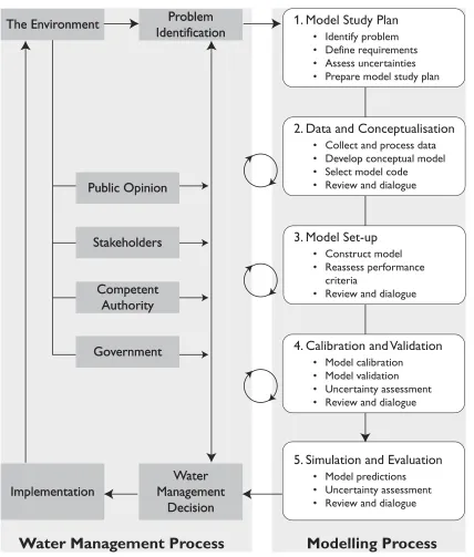
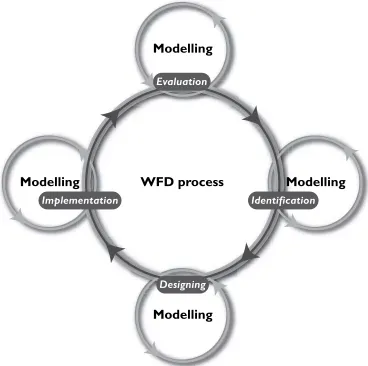
Models describing water flows, water quality, ecology and economy are being developed and used in increasing number and variety to support water management decisions. The interactions between the modelling process and the water management process are illustrated in Figs. 1 and 2. Fig. 1 shows the key actors in the water management process and the five steps that the modelling process typically may be decomposed in. The organisation that commissions a modelling study is denoted the water manager. This is often the competent authority, but can also be a stakeholder such as a water supply company. The role of the government is most often limited to providing the enabling environment such as legislation, research and information infrastructure. The typical cyclic and iterative character of the water management process, such as the WFD process, is illustrated in Fig. 2, where the interaction with the modelling process is illustrated by the large circle (water management) and the four smaller supporting circles (modelling). The WFD planning process, as most other planning processes, contains four main elements:

x Identification including assessment of present status, analysis of impacts and pressures and estab-lishment of environmental objectives. Here modelling may be useful for example for supporting as-sessments of what are the reference conditions and what are the impacts of the various pressures (EC, 2004).

x Designing including the set up and analysis of programme of measures designed to be able in a cost effective way to reach the environmental objectives. Here modelling will typically be used for supporting assessments of the effects and costs of various measures under consideration.

x Implementing the measures. Here on-line modelling in some cases may support the operational decisions to be made.

(14)

2. Data and Conceptualisation

• Collect and process data • Develop conceptual model • Select model code • Review and dialogue

3. Model Set-up

• Construct model • Reassess performance

criteria

• Review and dialogue

4. Calibration and Validation

• Model calibration • Model validation • Uncertainty assessment

5. Simulation and Evaluation

• Model predictions • Uncertainty assessment

1. Model Study Plan

• Identify problem • Define requirements • Assess uncertainties

• Prepare model study plan

Modelling Process

The Environment

Implementation

Problem

Identification

Problem

Identification

Water

Management

Decision

Water

Management

Decision

Public Opinion

Stakeholders

Competent

Authority

Competent

Authority

Government

Water Management Process

Fig. 1 The role of the modelling process and the water management decision process (inspired from Pascual et al. (2003).

(15)

x The modelling process starts with a thorough framing of the problem to be addressed and definition of modelling objectives and requirements for the modelling study (Step 1 in Fig. 1). Water manag-ers and stakeholdmanag-ers dominate this step, which basically is identical to part of the broader planning process. A participatory based assessment of the most important sources of uncertainty for the de-cision process should be used as a basis for prioritising the elements of the modelling study. The uncertainty assessments made at this stage will typically be qualitative.

x The main modelling itself is composed of steps 2, 3 and 4 of Fig. 1. Here the link with the main planning process consists of dialogue, reviews and discussions of preliminary results. The amount and type of interaction here depends on the level of public participation that may vary from case to case from providing information over consultation to active involvement (Henriksen et al., submit-ted).

x The finalisation of the modelling study (equivalent to the last step in Fig. 1), typically including sce-nario simulations. Here the water managers and the stakeholders again have a dominant role. The decisions made at the outcome of this step on the basis of modelling results are made in the con-text of the main planning process. Uncertainty assessment of model predictions is a crucial aspect of the modelling results and should be communicated in a way that is accessible for the stake-holders in the further water management process.

Modelling

WFD process

Modelling

Identification

Identification

Designing

Implementation

Evaluation

(16)

2.2 Terminology and Scientific Philosophical Basis for the Modelling

Process

2.2.1 Background

As pointed out in [12] a key problem in relation to establishment of a theoretical modelling framework is confusion on terminology. For example the terms validation and verification are used with different, and some times interchangeable, meanings by different authors. The confusion arises from both semantic and philosophical considerations (Rykiel, 1996). Another important problem is the lack of consensus related to the so far non-conclusive debate on the fundamental question concerning whether a water resources model can be validated or verified, and whether it as such can be claimed to be suitable or valid for particular applications (Konikow and Bredehoeft, 1992; De Marsily et al., 1992; Oreskes et al., 1994).

An important issue in relation to validation/verification is the distinction between open and closed sys-tems. A system is a closed system if its true conditions can be predicted or computed exactly. This ap-plies to mathematics and mostly to physics and chemistry. Systems where the true behaviour cannot be computed due to uncertainties and lack of knowledge on e.g. input data and parameter values are called open systems. The systems we are dealing with in water resources management, based on geo-sciences, biology and socio-economy, are open systems. According to Konikow and Bredehoeft (1992) and Oreskes et al. (1994) it is not possible to verify or validate models of open systems.

Finally, the principles have to reflect and be in line with the underlying philosophy of environmental modelling that have changed significantly during the past decades. In the early days many of us were focussing on the huge potentials of sophisticated models in a way that in retrospect may be character-ised as rather naive enthusiasm (e.g. Freeze and Harlan (1969); Abbott, 1992). The dominant views today appears to be a much more balanced and mature view (e.g. Beven, 2002a; Beven, 2002b).

2.2.2

Terminology and guiding principles

According to the terminology presented in [12] the simulation environment is divided into four basic elements as shown in Fig. 3. The inner arrows describe the processes that relate the elements to each other, and the outer circle refers to the procedures that evaluate the credibility of these processes.

In general terms a model is understood as a simplified representation of the natural system it attempts to describe. However, a distinction is made between three different meanings of the general term model, namely the conceptual model, the model code and the model that here is defined as a site-specific model. The most important elements in the terminology and their interrelationships are defined as follows:

Reality: The natural system, understood here as the study area.

(17)

simplifications and numerical accuracy limits that are assumed acceptable in order to achieve the purpose of the modelling. A conceptual model thus includes both a mathematical description (equations) and a descriptions of flow processes, river system elements, ecological structures, geological features, etc. that are required for the particular purpose of modelling. By drawing an analogy to scientific philosophical discussion the conceptual model in other words constitutes the scientific hypothesis or theory that we assume for our particular modelling study.

Fig. 3 Elements of a modelling terminology [12].

Model code: A mathematical formulation in the form of a computer program that is so generic that it, without program changes, can be used to establish a model with the same basic type of equations (but allowing different input variables and parameter values) for different study areas.

(18)

Model confirmation: Determination of adequacy of the conceptual model to provide an acceptable level of agreement for the domain of intended application. This is in other words the scientific confirmation of the theories/hypotheses included in the conceptual model.

Code verification: Substantiation that a model code is in some sense a true representation of a conceptual model within certain specified limits or ranges of application and corresponding ranges of accuracy.

Model calibration: The procedure of adjustment of parameter values of a model to reproduce the response of reality within the range of accuracy specified in the performance criteria.

Model validation: Substantiation that a model within its domain of applicability possesses a satisfactory range of accuracy consistent with the intended application of the model.

Model set-up: Establishment of a site-specific model using a model code. This requires, among other things, the definition of boundary and initial conditions and parameter assessment from field and laboratory data.

Simulation: Use of a validated model to gain insight into reality and obtain predictions that can be used by water managers. This includes insight into how reality can be expected to respond to human interventions. In this connection uncertainty assessments of the model predictions are very important.

Performance criteria: Level of acceptable agreement between model and reality. The performance criteria apply both for model calibration and model validation.

Domain of applicability (of conceptual model): Prescribed conditions for which the conceptual model has been tested, i.e. compared with reality to the extent possible and judged suitable for use (by model confirmation).

Domain of applicability (of model code): Prescribed conditions for which the model code has been tested, i.e. compared with analytical solutions, other model codes or similar to the extent possible and judged suitable for use (by code verification).

Domain of applicability (of model): Prescribed conditions for which the site-specific model has been tested, i.e. compared with reality to the extent possible and judged suitable for use (by model valida-tion).

2.2.3 Scientific

philosophical

aspects

(19)

model is eventually accepted as valid for specific conditions, this is not a proof that the conceptual model is true, because, due to non-uniqueness, the site-specific model may turn out to perform right for the wrong reasons.

The fundamental view expressed by scientific philosophers is that verification and validation of numeri-cal models of natural systems is impossible, because natural systems are never closed and because the mapping of model results are always non-unique (Popper, 1959; Oreskes et al., 1994). I agree that it is not possible to carry out model verification or model validation, if these terms are used universally, without restriction to domains of applicability and levels of accuracy.

[12] note, however, that Popper (1959) distinguished between two kinds of universal statements: the 'strictly universal' and the 'numerical universal'. The strictly universal statements are those usually dealt with when speaking about theories or natural laws. They are a kind of 'all-statement' claiming to be true for any place and any time. In contrary, numerical universal statements refers only to a finite class of specific elements within a finite individual spatio-temporal region. A numerical universal statement is thus in fact equivalent to conjunctions of singular statements.

The restrictions in use of the terms confirmation, verification and validation imposed by the respective domains of applicability imply, according to Popper's views, that the conceptual model, model code and site-specific models can only be classified as numerical universal statements as opposed to strictly uni-versal statements. This distinction is fundamental for the terminology described in [12] and its link to scientific philosophical theories. Consequently the terms verification and validation should never be used without qualifiers.

(20)

2.3 Modelling Protocol

The procedure for applying a hydrological model is often denoted a modelling protocol. It comprises a series of actions to be followed in a sequential or iterative form. The modelling protocol presented in [7] for distributed catchment modelling was inspired by the groundwater community (Anderson and Woessner, 1992). It was subsequently used in the Danish Handbook for Groundwater Modelling (Hen-riksen et al., 2001) that has been used extensively in practise since its emergence. A more recent mod-elling protocol, developed within the context of the EU research project HarmoniQuA, is reported in [13] and Scholten et al. (2007). The two protocols are illustrated in Figs. 4 and 5.

(21)

A modelling study will involve several phases and several actors. A typical modelling study will involve the following four different types of actors:

x The water manager, i.e. the person or organisation responsible for the management or protection of the water resources, and thus responsible for the modelling study and the outcome (the problem owner).

x The modeller, i.e. a person or an organisation that works with the model conducting the modelling study. If the modeller and the water manager belong to different organisations, their roles will typi-cally be denoted consultant and client, respectively.

x The reviewer, i.e. a person that is conducting some kind of external review of a modelling study. The review may be more or less comprehensive depending on the requirements of the particular case. The reviewer is typically appointed by the water manager to support the water manager to match the modelling capability of the modeller.

x The stakeholders/public. A stakeholder is an interested party with a stake in the water management issue, either in exploiting or protecting the resource. Stakeholders include the following different groups: (i) competent water resource authority (typically the water manager, cf. above); (ii) interest groups; and (iii) general public.

The modelling process may, according to [13], be decomposed into five major steps which again are decomposed into 48 tasks (Fig. 5). The contents of the five steps are:

x STEP1 (Model Study Plan). This step aims to agree on a Model Study Plan comprising answers to the questions: Why is modelling required for this particular model study? What is the overall model-ling approach and which work should be carried out? Who will do the modelmodel-ling work? Who should do the technical reviews? Which stakeholders/public should be involved and to what degree? What are the resources available for the project? The water manager needs to describe the problem and its context as well as the available data. A very important task is then to analyse and determine the various requirements of the modelling study in terms of the expected accuracy of modelling results. The acceptable level of accuracy will vary from case to case and must be seen in a socio-economic context. It should, therefore, be defined through a dialogue between the modeller, water manager and stakeholders/public. In this respect an analysis of the key sources of uncertainty is crucial in order to focus the study on the elements that produce most information of relevance to the problem at hand.

x STEP 2 (Data and Conceptualisation). In this step the modeller should gather all the relevant knowledge about the study basin and develop an overview of the processes and their interactions in order to conceptualise how the system should be modelled in sufficient detail to meet the require-ments specified in the Model Study Plan. Consideration must be given to the spatial and temporal detail required of a model, to the system dynamics, to the boundary conditions and to how the model parameters can be determined from the available data. The need to model certain processes in alternative ways or to differing levels of detail in order to enable assessments of model structure uncertainty should be evaluated. The availability of existing computer codes that can address the model requirements should also be addressed.

(22)

up the generation of input files, but it does not guarantee that the input files are error free. The modeller performs this work.

x STEP 4 (Calibration and Validation). This step is concerned with the process of analysing the model that was constructed during the previous step, first by calibrating the model, and then by validating its performance against independent field data. Finally, the reliability of model simulations for the in-tended domain of applicability is assessed through uncertainty analyses. The results are described so that the scope of model use and its associated limitations are documented and made explicit. The modeller performs this work.

x STEP 5 (Simulation and Evaluation). In this step the modeller uses the calibrated and validated model to make simulations to meet the objectives and requirements of the model study. Depending on the objectives of the study, these simulations may result in specific results that can be used in subsequent decision making (e.g. for planning or design purposes) or to improve understanding (e.g. of the hydrological/ecological regime of the study area). It is important to carry out suitable un-certainty assessments of the model predictions in order to arrive at a robust decision. As with the other steps, the quality of the results needs to be assessed through internal and external reviews. Each of the last four steps is concluded with a reporting task followed by a review task. The review tasks include dialogues between water manager, modeller, reviewer and, often, stakeholders/public. The protocol includes many feedback possibilities (Fig. 5).

A comparison of the old protocol (Fig. 4) and the one decade younger HarmoniQuA protocol (Fig. 5) shows some interesting developments:

x The basic sequence of the prescribed activities in the protocols is the same. The HarmoniQuA pro-tocol is much more detailed than the old one, but there are no fundamental disagreements be-tween the two.

x The HarmoniQuA protocol puts much more emphasis on the framing of the modelling study. This is only considered in one box in Fig. 4 and not given much weight in [7], while it is one full Step comprising seven tasks in Fig 5. This implies for instance that requirements on performance crite-ria and uncertainty assessments are introduced rather late in the old protocol, while it is an impor-tant part of Step 1 in the HarmoniQuA protocol.

x There is much emphasis on uncertainty assessments throughout the modelling process in the HarmoniQuA protocol, while uncertainty assessments are only considered as part of model cali-bration and simulation in the old protocol.

x The HarmoniQuA protocol is part of a quality assurance framework with much emphasis on the role play between the various actors in the modelling process. This results in stakeholder involve-ment, peer reviews, focus on reporting and dialogue between water manger and modeller. In con-trary to this, the old protocol only focuses on the modeller.

(23)

Specify or Update Calibration and Validation Targets and Criteria Test Runs Completed Model Set-up Construct Model OK Dire

Dire Not OK

OK

Not OK

Review Model Set-up and Calibration

and Validation Plan Report and Revisit Model

Study Plan (Model Set-up) Model Study Plan

Describe Problem and Context

Proposal and Tendering Prepare Terms of

Reference Determine Requirements Identify Data Availability Define Objectives Yes No _{Agree on}

Model Study Plan and Budget

Collect and Process Raw Data Sufficient Data? Code Selection Assess Soundness of Conceptualis-ation Process Model Structure Data Model Structure and

Processes Need for Alternative Conceptual Models? Model Parameters Summarise Conceptual Model and

Assumptions No Yes Dire Yes No Dire OK OK Not OK Not OK

Review Data and Conceptualisation and

Model Set-up Plan Report and Revisit

Model Study Plan (Data and Conceptualisation)

Validation

Uncertainty Analysis of Calibration and

Validation

Scope of Applicability Assess Soundness of Validation Assess Soundness of Calibration Method

Define Stop Criteria

Select Calibration Parameters Parameter Estimation All Calibration Stages Completed? OK Not OK Yes No Dire OK Not OK OK Not OK Not OK OK Review Calibration and Validation

and Simulation Plan Report and Revisit Model Study Plan (Calibration and

Validation)

Dire

Analyse and Interpret Results Uncertainty Analysis of Simulation Simulations Reporting of Simulation and Evaluation Check Simulations Assess Soundness of Simulattion

Need for Post Audit

Not OK OK Not OK Dire Not OK OK Review of Simulation and Evaluation OK Model Study Closure Set-up Scenario All Scenarios Completed? No Yes

Specify or Update Calibration and Validation Targets and Criteria Test Runs Completed Model Set-up Construct Model OK Dire

Dire Not OK

OK

Not OK

Review Model Set-up and Calibration

and Validation Plan Report and Revisit Model

Study Plan (Model Set-up) Specify or Update

Calibration and Validation Targets and Criteria Test Runs Completed Test Runs Completed Model Set-up Construct Model OK Dire

Dire Not OK

OK

Not OK

Review Model Set-up and Calibration

and Validation Plan Review Model Set-up and Calibration

and Validation Plan Report and Revisit Model

Study Plan (Model Set-up) Model Study Plan

Proposal and Tendering Prepare Terms of

Model Study Plan and Budget Model Study Plan

Proposal and Tendering Prepare Terms of

Model Study Plan and Budget

Agree on Model Study Plan

and Budget

Collect and Process Raw Data Sufficient Data? Code Selection Assess Soundness of Conceptualis-ation Process Model Structure Data Model Structure and

Processes Need for Alternative Conceptual Models? Model Parameters Summarise Conceptual Model and

Model Study Plan (Data and Conceptualisation) Collect and Process

Raw Data Sufficient Data? Sufficient Data? Code Selection Assess Soundness of Conceptualis-ation Assess Soundness of Conceptualis-ation Process Model Structure Data Model Structure and

Processes Need for Alternative Conceptual Models? Need for Alternative Conceptual Models? Model Parameters Summarise Conceptual Model and

Model Set-up Plan Review Data and Conceptualisation and

Model Study Plan (Data and Conceptualisation)

Validation

Uncertainty Analysis of Calibration and

Validation

Scope of Applicability Assess Soundness of Validation Assess Soundness of Calibration Method

Select Calibration Parameters Parameter Estimation All Calibration Stages Completed? OK Not OK Yes No Dire OK Not OK OK Not OK Not OK OK Review Calibration and Validation

Validation)

Dire

Validation

Uncertainty Analysis of Calibration and

Validation

Scope of Applicability Assess Soundness of Validation Assess Soundness of Validation Assess Soundness of Calibration Assess Soundness of Calibration Method

Select Calibration Parameters Parameter Estimation Parameter Estimation All Calibration Stages Completed? All Calibration Stages Completed? OK Not OK Yes No Dire OK Not OK OK Not OK Not OK OK Review Calibration and Validation

and Simulation Plan Review Calibration and Validation

Validation)

Dire

Analyse and Interpret Results Uncertainty Analysis of Simulation Simulations Reporting of Simulation and Evaluation Check Simulations Assess Soundness of Simulattion

Not OK OK Not OK Dire Not OK OK Review of Simulation and Evaluation OK Model Study Closure Set-up Scenario All Scenarios Completed? No Yes

Analyse and Interpret Results Uncertainty Analysis of Simulation Simulations Reporting of Simulation and Evaluation Check Simulations Check Simulations Assess Soundness of Simulattion Assess Soundness of Simulattion

Not OK OK Not OK Dire Not OK OK Review of Simulation and Evaluation Review of Simulation and Evaluation OK Model Study Closure Set-up Scenario All Scenarios Completed? All Scenarios Completed? No Yes

(24)

2.4 Classification of Models

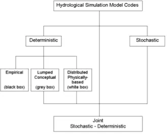
Many attempts have been made to classify hydrological models (or model codes). Refsgaard (1996) presented the classification shown in Fig. 6 that I have used in all papers of the present thesis. Deter-ministic models can be classified according to whether the model gives a lumped or a distributed de-scription of the considered area, and whether the dede-scription of the hydrological processes is empirical, conceptual, or more physically-based. A lumped model implies that the catchment is considered as one computational unit. A distributed model, on the other hand, provides a description of catchment proc-esses at geo-referenced computational grid points within the catchment. An intermediate approach is a semi-distributed model, which uses some kind of distribution, either in sub-catchments or in hydrologi-cal response units, where areas with the same key characteristics are aggregated to sub-units without considering their actual locations within the catchment. Examples of hydrological response units con-sidered in semi-distributed models are elevation zones, which are relevant for snow modelling, and combinations of soil and vegetation type, which may be relevant for simulation of root zone processes such as evapotranspiration and nitrate leaching.

As most conceptual models are also lumped, and as most physically-based models are also distributed, the three main classes emerge:

x Empirical (black box)

x Lumped conceptual models (grey box)

x Distributed physically-based (white box)

(25)

Fig. 6 Classification of hydrological models according to process description (Refsgaard, 1996).

Typical examples of lumped conceptual model codes are the Stanford Watershed Model (Crawford and Linsley, 1966), the Sacramento (Burnash, 1995), the HBV (Bergström, 1995) and the NAM (Nielsen and Hansen, 1973). Typical examples of distributed physically-based model codes are the MIKE SHE (Abbott et al., 1986a, b; Refsgaard and Storm, 1995) and the Thales (Grayson et al., 1992a, b). Groundwater model codes like MODFLOW belong to the distributed physically-based class.

(26)

3 Simulation of Hydrological Processes at Catchment

Scale

In this chapter some modelling examples from the publications are briefly summarised and discussed within the framework outlined in Chapter 2.

3.1 Flow modelling

3.1.1

Groundwater/surface water model for the Suså catchment ([1], [2])

Summary

The publications [1] and [2] describe a new model code and the set-up, calibration and validation of a model for a 1,000 km2 area. Further details can be found in Stang (1981), Refsgaard (1981) and Refsgaard and Stang (1981). The objectives of the study were to develop a spatially distributed groundwater/surface water model code and apply it to the Suså catchment with a particular focus on the stream-aquifer interaction in a hydrogeological system consisting of confined aquifer-aquitard-phreatic aquifer and to test the model for prediction of the hydrological consequences on streamflows and hydraulic heads of groundwater abstraction.

The new model code was rather complex and computationally demanding at the time of development. Thus, standard 30 years model simulations could only be carried out as night runs at the main frame computer at DTU’s computer centre.

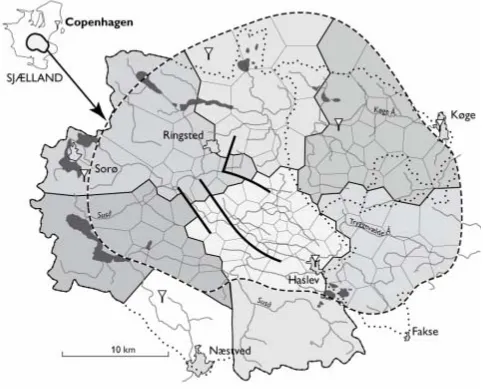
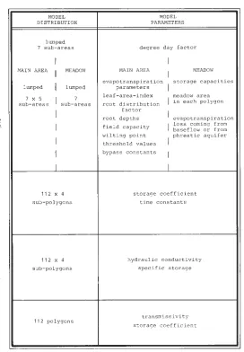
The model area comprising the Suså and the neighbouring Køge Å catchments is located in the central and southern part of Zealand. The model area, the topographic divides and the groundwater model polygonal mesh are shown in Fig. 7. The overall structure of the model is outlined in Fig. 8. It consists of four separate components for the confined regional aquifer, the aquitard, the phreatic aquifer and the root zone. The spatial distribution and the degree of physical basis differ between the four components. The time steps in the calculations are one day in all parts of the model.

(27)

The root zone component calculated the net precipitation that recharged the phreatic aquifer. The mod-elling area was divided into seven sub-areas with separate precipitation input and soil parameters. Fur-ther the spatial variation in vegetation was accounted for by dividing each of these seven areas into five vegetation areas based on agricultural statistics and one meadow (wetland) area. This makes the total distribution to 42 sub-areas where each sub-area is a kind of ‘hydrological response unit’, i.e. a semi-distributed approach. The root zone calculations were based on a box approach with four layers in the root zone.

(28)

Fig. 8 The structure of the Suså model

40

30

20

10

0

0 1 2 3

km

50 100 %

Lilleå

Legend

< 24 m above MSL 24–28 m above MSL 28–34 m above MSL > 34 m above MSL

Suså

Vendebæk

Gasmose Bæk

POLYGON 21

1

1 22 33 44 Aquitard

Ground surface

Water table (lower outlet)

Head, regional aquifer

Pre-Quaternary surface

Regional aquifer

(29)

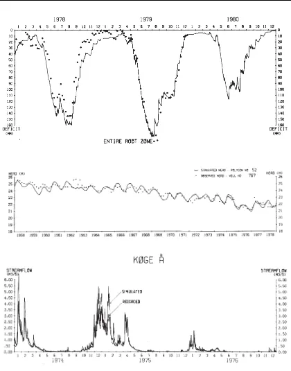
Fig. 10 Examples of simulation results from soil moisture in root zone, hydraulic head of regional con-fined aquifer and river discharge.

(30)

were calibrated against only some of the available streamflow data, namely some of the data from the Suså catchment, while amongst others Køge Å data were not used for calibration.

While the simulation of streamflows in the Køge Å catchment in [1] was characterised as a “half-way test of the model’s ability to simulate streamflow from ungauged catchments” no systematic validation tests against independent data were carried out as part of the study. Some years later the model simu-lations were extended with new data from the period 1981-87, where the groundwater abstractions had changed slightly. In this post audit validation study the model simulations were found to match the ob-servations to the same degree of accuracy as during the calibration period (Jensen and Jørgensen, 1988).

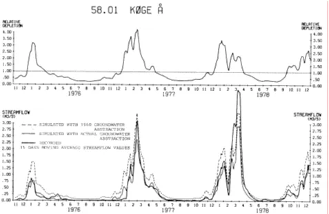
The model’s ability to simulate the streamflow depletion caused by a groundwater abstraction from the regional confined aquifer was tested on historical data from the Køge Å catchment. Fig. 11 shows simu-lated streamflow assuming actual groundwater abstraction from the Regnemark Waterworks starting in 1964, Qsim, and assuming no abstracting from Regnemark, Q1sim. The recorded streamflow fits

rea-sonably well with Qsim. The difference Q1sim - Qsim, which is the simulated streamflow depletion caused

by the increased groundwater abstraction, is seen to have a clear seasonal variation with smaller deple-tion during the dry summer periods and larger depledeple-tion during the wet winter season.

(31)

Discussion - post evaluation

Most other catchment models existing when the Suså model code was developed were either purely rainfall runoff models of the lumped conceptual type, such as the classical Stanford Watershed Model (Crawford and Linsley, 1966), the HBV (Bergström and Forsman, 1973; Bergström, 1976) and the NAM (Nielsen and Hansen, 1973) or purely groundwater models (Prickett and Lonnquist, 1971; Thomas, 1973). A few authors had concluded that coupled groundwater/surface water modelling was essential (e.g. Luckner, 1978; Lloyd, 1980) and some had outlined specific, but not yet operational, concepts (e.g. Freeze and Harlan, 1969; Wardlaw, 1978; Jønch-Clausen, 1979). In some studies groundwater models and rainfall-runoff models were used at the same catchment, but without coupling (e.g. Weeks et al., 1974). Thus, apparently no other model had previously been used to dynamically simulate cou-pled groundwater/surface water conditions at catchment scale (rainfall, evapotranspiration, surface near runoff, groundwater recharge, groundwater heads, baseflow discharge from aquifers to streams).

During the decade following [1] and [2] a few model codes with integrated groundwater/surface water descriptions emerged. The most prominent of these codes was the SHE (Abbott et al., 1986a, b) and its operational daughter codes, MIKE SHE from DHI (Refsgaard and Storm, 1995) and SHETRAN from University of Newcastle (Bathurst and O’Connell, 1992), which both are used today, although in later versions. Other operational models from that period were described by Miles and Rushton (1983), Christensen (1994) and Wardlaw (1994). Miles and Rushton (1983) used a simpler root zone and sur-face water component than [1] together with a two-dimensional finite difference groundwater model and monthly time steps. Christensen (1994) developed a model for the Tude Å catchment (a neighbour to Suså) that conceptually was similar and a little bit simpler than [1]. Wardlaw et al. (1994) used the con-cepts outlined in Wardlaw (1978) coupling the Stanford Watershed Model with a finite-difference groundwater model and a channel routing model for simulation of discharge and groundwater levels in the Allen catchment in England.

During the past decade the number of integrated modelling codes has exploded. The existing codes today can be considered to fall in three classes: (a) fully integrated codes such as MIKE SHE (Graham and Butts, 2005); (b) couplings of existing groundwater codes and surface water codes such as MOD-FLOW and SWAT (Perkins and Sophocleous, 1999); and (c) codes based on the fully 3-dimensional Richards’ equation (Panday and Hayakorn, 2004). Independent reviews of the scientific basis and prac-tical applicability of a number of recent integrated model codes are provided by e.g. Kaiser-Hill (2001) and Tampa Bay Water (2001).

(32)

catch-ments in connection with groundwater abstraction was Christensen (1994) who basically confirmed the results of [2].

The spatial distribution and the degree of physical basis differ between the four components of the Suså model. The groundwater model can be characterised as distributed physically-based, the aquitard model as distributed physically-based and the phreatic aquifer and root zone models as semi-distributed conceptual. In contrary to for instance the later SHE code (Abbott et al, 1986a, b), the Suså model code was not generic, because it could not be applied to other catchments without changes in the code. Furthermore, it was tailored to the specific hydrological conditions prevailing in the Suså catchment and could for instance not be applied to an alluvial unconfined aquifer.

In retrospect, it is interesting to observe that issues related to the credibility of model simulations were not critically analysed or discussed in [1] and [2]. First of all, aspects of code verification were not dealt with in the publications, although a major novelty of the work was the development of a completely new code. Secondly, and maybe more surprisingly, model validation and uncertainty assessments of model simulations were almost not addressed. By using all the available groundwater head data for calibration the opportunity to make split-sample validation test against parts of the data or even the unique oppor-tunity to calibrate on data before the groundwater abstraction and validate on data after the abstraction (differential split-sample test according to Klemes (1986)) were not utilised. By not addressing the un-certainty and by not conducting rigorous validation tests the reader may be left with the, undocumented, impression that the curve fitting in Fig. 10 is supposed to reflect the predictive capability of the model. That the model proved to perform well in a subsequent post-audit validation study could not be known at the time of [1] and [2].

(33)

3.1.2

Application of SHE to catchments in India ([4], [5])

Summary

The publications [4] and [5] describe the set-up, calibration and validation of the ‘Système Hydrologique Européen’ (SHE) code to six sub-catchments totalling about 15,000 km2_{of the Narmada basin in India,}

Fig. 12. The objective of the papers was to describe experiences from applying a distributed physically-based code like SHE to large basins with rather limited data coverage compared to previous SHE ap-plications to research catchments. In contrary to the Suså study in [1] and [2], the India study did not include any code development, except for data processing utility software. Instead it comprised applica-tion of an existing code (Abbott et al., 1986a,b) to condiapplica-tions that were far beyond the condiapplica-tions for which the SHE had previously been tested in terms of catchment size, data coverage and hydrological regime (Bathurst, 1986a).

Fig. 12 Location map for the Narmada and the six sub-catchments.

(34)

The data requirements for a SHE based model is substantial and much larger than for a rainfall-runoff model of lumped conceptual type that previously had been applied to such types of catchments. A ma-jor challenge of the study was therefore to identify, collect and process data and to check their quality. Data were collected from more than 15 different agencies belonging to many different ministries and the data quality varied substantially.

Another challenge was how to assess parameter values in a distributed model when data, in contrary to the previous tests on small experimental catchments like in Bathurst (1986a), are scarce. Each of the grid points in a distributed model is characterised by one or more parameters. Although the parameter values in principle (as in nature) vary from grid point to grid point, it is neither feasible nor desirable to allow the parameter values to vary so freely. Instead, a given parameter should only reflect the significant and systematic variation described in the available field data. Therefore a parameterisation procedure was developed, where representative parameter values were associated to individual soil types, vegetation types, geological layers, etc. This process of defining the spatial pattern of parameter values effectively reduced the number of free parameter coefficients, which needs to be adjusted in the subsequent calibration procedure. For example, the 820 km2 Kolar catchment is parameterised into three soil classes and 10 land use/soil depth classes. For the soil type classes calibration was allowed for the hydraulic conductivity in the unsaturated zone (for each soil type class the conductivity could vary among three different land uses => nine parameter values). For the land use/soil depth classes the calibration parameters comprised soil depths (10 parameters in total) and the Strictler overland flow coefficients for four land use types (four parameters in total). Further three parameters were subject to calibration (hydraulic conductivity in the saturated zone, an (empirical) by-pass coefficient and a surface retention parameter; all kept constant throughout the catchment). Although the 26 calibration parameters could not be assessed from field data alone, but had to be modified through calibration, the physical realism of the parameter values resulting from the subsequent calibration procedure could be evaluated from available field data.

The simulation results are illustrated in Fig. 13 as hydrographs for the largest sub-catchment and in Fig. 14 as annual runoff and annual peaks for all six sub-catchments. In both figures the results are for the validation periods, where results are slightly poorer as compared to the calibration periods. In [4] the rainfall-runoff simulation results were characterised as having the same degree of accuracy as would have been expected with simpler hydrological models of the lumped conceptual type. The results there-fore suggested that application of complex data demanding models like the present SHE approach are not justified in cases where the modelling objective is limited to simulation of catchment runoff and where observed runoff records exist for calibration purposes. No attempts were made in the study to test the capability of a model without calibration.

(35)

Fig. 13 Observed and simulated hydrographs for the Narmada at Manot during the validation period 1985 and 1987.

(36)

Discussion - post evaluation

At the time of [4] and [5] lumped conceptual catchment model codes such as HBV (Bergström, 1992) and NAM (Jønch-Clausen and Refsgaard, 1984) had been used operationally for two decades, typically for catchments ranging from a few km2 to more than 10,000 km2.

At the same time distributed physically-based models had mainly been tested on flood events on small catchments that typically had very good data due to experimental instrumentation (Loague and Freeze, 1985; Bathurst 1986a; Grayson et al., 1992a,b; Troch et al., 1993). Loague and Freeze (1985) com-pared a quasi-physically based model with a regression model and a unit hydrograph model on three experimental catchments, the 0.1 km2 R-5, Chickasha, Oklahoma, the 7.2 km2 WE-38, Klingertown, Pensylvania and the 0.1 km2 HB-6, West Thornton, New Hampshire. Bathurst (1986a) applied the SHE to the simulation of flood events for the 10.6 km2_{experimental Wye catchment in Wales. Grayson et al.}

(1992a,b) applied the THALES to the simulation of flood events for the 7.0 ha Wagga catchment in Aus-tralia and the 4.4 ha Lucky Hill catchment at the Walnut Gulch Experimental Area in Arizona. Troch et al. (1993) applied a model based on a 3-dimensional numerical solution to Richards’ equation to the 7.2 km2_{WE-38 catchment and a 0.64 km}2_{subcatchment.}

To my knowledge the only examples until then of distributed physically-based model studies including applications on several hundred km2_{catchments and continuous simulation for periods of several years}

were the coupled groundwater/surface water models discussed in the previous section ([1]; [2]; Miles and Rushton, 1983; Christensen, 1994; Wardlaw et al., 1994) that all had distributed physically-based groundwater components and lumped (or semi-distributed) conceptual surface water components and some models such as WATBAL (Knudsen et al., 1986) that had semi-distributed surface water compo-nents and lumped conceptual groundwater compocompo-nents.

During the following few years a few additional catchment scale studies with continuous simulations of distributed physically-based models emerged. One example is Querner (1997) who applied the MOGROW to the 6.5 km2 Hupselse Beek catchment simulating both discharge and groundwater head dynamics. Another example is Kutchment et al. (1996) who simulated surface water processes for the 3315 km2_{Ouse catchment. The study of Kutchment et al (1996) had many similarities with [4] and [5]}

with respect to model conceptualisation and conclusions.

The main scientific contribution of [4] and [5] was therefore as the first study to demonstrate that distrib-uted physically-based models could be established for catchments of this size and with ordinary data availability. Previous studies reported in literature had either been tests on small research catchments or been models with major components of the lumped conceptual type. As outlined above, it is worth noting the different traditions in the communities that had dealt with (large scale) lumped conceptual models, (small scale) physically-based models and groundwater models, respectively. I believe that an important characteristic of the team who performed the present study ([4] and [5]) was that it comprised scientists who together had comprehensive experiences from all these communities.

(37)

in [1], it is still very high and it is very likely that a sensitivity analysis would have shown that this num-ber could easily be reduced without loss of model performance. It is interesting to note that similar pa-rameterisation approaches reported for other catchments in 1997 ([7]) and 2001 (Andersen et al., 2001) resulted in 11 and 4 free parameters, respectively, implying that the parameterisation approach adopted in [4] and [5] were not yet finally developed.

Beven (1989) had provided a fundamental critique of the way physically-based models such as the SHE had been promoted by e.g. Abbott et al. (1986a) and Bathurst (1986a). His main critique was that the attitudes in these early SHE papers were not realistic with respect to the abilities and achievements of physically-based models. Beven pointed amongst others to the following key problems:

x The process equations are simplifications leading to model structure uncertainty.

x Spatial heterogeneity at subgrid scale is not included in the physically-based models. The current generation of distributed physically-based models are in reality lumped conceptual models.

x There is a great danger of overparameterisation if it is attempted to simulate all hydrological proc-esses thought to be relevant and the related parameters against observed discharge data only. As a conclusion Beven argued that for future applications attempts must be made to obtain realistic estimates of the uncertainty associated with their predictions, particularly in the case of evaluating fu-ture scenarios of the effects of management strategies.

[4] noted some of Beven’s critique, acknowledging that the process representation at the 2 km x 2 km grid squares is causing significant violations of some of the process descriptions, that “some degree of lumping and conceptualisation has taken place at the grid scale” and that “scale problems are impor-tant”. [4] stressed, however, that in spite of these acknowledged limitations “the present basin model is much more physically based and distributed than the traditional lumped conceptual model, where the entire catchment is represented in effect by one grid square, and where the process representations due to averaging over characteristics of topography, soil type and vegetation type are fundamentally different from the basic physical laws”.

[4] and [5] concluded that the SHE is a suitable tool to support water management for conditions in In-dia. In contrary to this, Beven (1989) had stated that the physically-based models “are not well suited to applications to real catchments”. In retrospect, it is remarkable that [4] and [5] did not go more substan-tially into a dialogue with the very fundamental critique raised by Beven (1989). For instance [4] and [5] did not comment at all on Beven’s main conclusion on the need for uncertainty assessment, although [5] actually used the model to study the impact of soil and land use by performing sensitivity analyses. A more comprehensive response and dialogue took place a few years later (Beven, 1996a; Refsgaard et al., 1996; Beven, 1996b).

(38)

3.1.3

Intercomparison of different types of hydrological models ([6])

Summary

The research study reported in publication [6] had two objectives. The first objective was to identify a rigorous framework for the testing of model capabilities for different types of tasks. The second objec-tive was to use this theoretical framework and conduct an intercomparison study involving application of three model codes of different complexity to a number of tasks ranging from traditional simulation of stationary, gauged catchments to simulation of ungauged catchments and of catchments with nonsta-tionary climate conditions. Data from three catchments in Zimbabwe were used for the tests.

The three codes used in the study were (a) NAM (Nielsen and Hansen, 1973; Havnø et al., 1995) – Fig. 15; (b) WATBAL (Knudsen et al., 1986) – Fig. 16; and (c) MIKE SHE (Abbott et al., 1986a,b; Refsgaard and Storm, 1995) – Fig. 17. The NAM and MIKE SHE can be characterised as very typical of their lumped conceptual and distributed physically-based types, respectively, while the WATBAL with its semi-distributed approach falls in between these two standard classes.

(39)

Fig. 16 Structure of the WATBAL code.

Fig. 17 Schematic representation of the model structure of the ‘Système Hydrologique Européen’ (SHE) code.

(40)

The model performance was evaluated for annual runoff and criteria focussing on the shape of the dis-charge hydrograph, i.e. rainfall-runoff modelling. The modelling work was carried out by three different persons/teams that were very experienced by applying their respective model codes. A general conclu-sion from the study was that the performances of the three codes were surprisingly similar. Thus, the ability of WATBAL and SHE to explicitly utilise data such as topography, soil and vegetation data that the NAM could not use turned out to make no significant difference in most cases. In summary the con-clusions were:

x Given a few (1–3) years of runoff measurements, a lumped model of the NAM type would be a suitable tool from the point of view of technical and economical feasibility. This applies for catch-ments with homogeneous climatic input as well as cases where significant variations in the exoge-nous input are encountered.

x For ungauged catchments, however, where accurate simulations are critical for water resources decisions, a distributed model is expected to give better results than a