Mathematical Background:
Foundations of Infinitesimal Calculus
second editionby K. D. Stroyan
x y
y=f(x)
dx dy
δx ε
dx dy
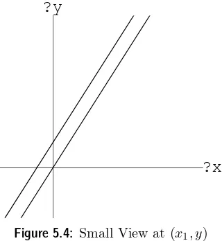
Figure 0.1: A Microscopic View of the Tangent
Copyright c1997 by Academic Press, Inc. - All rights reserved.
i
Preface to the Mathematical Background
We want you to reason with mathematics. We are not trying to get everyone to give formalized proofs in the sense of contemporary mathematics; ‘proof’ in this course means ‘convincing argument.’ We expect you to use correct reasoning and to give careful expla-nations. The projects bring out these issues in the way we find best for most students, but the pure mathematical questions also interest some students. This book of mathemat-ical “background” shows how to fill in the mathematmathemat-ical details of the main topics from the course. These proofs are completely rigorous in the sense of modern mathematics – technically bulletproof. We wrote this book of foundations in part to provide a convenient reference for a student who might like to see the “theorem - proof” approach to calculus.
We also wrote it for the interested instructor. In re-thinking the presentation of beginning calculus, we found that a simpler basis for the theory was both possible and desirable. The pointwise approach most books give to the theory of derivatives spoils the subject. Clear simple arguments like the proof of the Fundamental Theorem at the start of Chapter 5 below are not possible in that approach. The result of the pointwise approach is that instructors feel they have to either be dishonest with students or disclaim good intuitive approximations. This is sad because it makes a clear subject seem obscure. It is also unnecessary – by and large, the intuitive ideas work provided your notion of derivative is strong enough. This book shows how to bridge the gap between intuition and technical rigor.
A function with a positive derivative ought to be increasing. After all, the slope is positive and the graph is supposed to look like an increasing straight line. How could the function NOT be increasing? Pointwise derivatives make this bizarre thing possible - a positive “derivative” of a non-increasing function. Our conclusion is simple. That definition is WRONG in the sense that it does NOT support the intended idea.
You might agree that the counterintuitive consequences of pointwise derivatives are un-fortunate, but are concerned that the traditional approach is more “general.” Part of the point of this book is to show students and instructors that nothing of interest is lost and a great deal is gained in the straightforward nature of the proofs based on “uniform” deriva-tives. It actually is not possible to give a formula that is pointwise differentiable and not uniformly differentiable. The pieced together pointwise counterexamples seem contrived and out-of-place in a course where students are learning valuable new rules. It is a theorem that derivatives computed by rules are automatically continuous where defined. We want the course development to emphasize good intuition and positive results. This background shows that the approach is sound.
This book also shows how the pathologies arise in the traditional approach – we left pointwise pathology out of the main text, but present it here for the curious and for com-parison. Perhaps only math majors ever need to know about these sorts of examples, but they are fun in a negative sort of way.
ii
derivatives, although this can also be clearly understood using function limits as in the text by Lax, et al, from the 1970s. Modern graphical computing can also help us “see” graphs converge as stressed in our main materials and in the interesting Uhl, Porta, Davis,Calculus & Mathematicatext.
Almost all the theorems in this book are well-known old results of a carefully studied subject. The well-known ones are more important than the few novel aspects of the book. However, some details like the converse of Taylor’s theorem – both continuous and discrete – are not so easy to find in traditional calculus sources. The microscope theorem for differential equations does not appear in the literature as far as we know, though it is similar to research work of Francine and Marc Diener from the 1980s.
We conclude the book with convergence results for Fourier series. While there is nothing novel in our approach, these results have been lost from contemporary calculus and deserve to be part of it. Our development follows Courant’s calculus of the 1930s giving wonderful results of Dirichlet’s era in the 1830s that clearly settle some of the convergence mysteries of Euler from the 1730s. This theory and our development throughout is usually easy to apply. “Clean” theory should be the servant of intuition – building on it and making it stronger and clearer.
Contents
Part 1
Numbers and Functions
Chapter 1. Numbers 3
1.1 Field Axioms 3
1.2 Order Axioms 6
1.3 The Completeness Axiom 7 1.4 Small, Medium and Large Numbers 9 Chapter 2. Functional Identities 17 2.1 Specific Functional Identities 17 2.2 General Functional Identities 18 2.3 The Function Extension Axiom 21 2.4 Additive Functions 24 2.5 The Motion of a Pendulum 26
Part 2 Limits
Chapter 3. The Theory of Limits 31
3.1 Plain Limits 32
3.2 Function Limits 34
3.3 Computation of Limits 37 Chapter 4. Continuous Functions 43 4.1 Uniform Continuity 43 4.2 The Extreme Value Theorem 44
iv Contents
4.3 Bolzano’s Intermediate Value Theorem 46
Part 3
1 Variable Differentiation
Chapter 5. The Theory of Derivatives 49 5.1 The Fundamental Theorem: Part 1 49
5.1.1 Rigorous Infinitesimal Justification 52
5.1.2 Rigorous Limit Justification 53
5.2 Derivatives, Epsilons and Deltas 53 5.3 Smoothness⇒ Continuity of Function and Derivative 54 5.4 Rules⇒ Smoothness 56 5.5 The Increment and Increasing 57 5.6 Inverse Functions and Derivatives 58 Chapter 6. Pointwise Derivatives 69
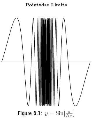
6.1 Pointwise Limits 69
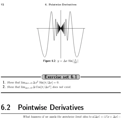
6.2 Pointwise Derivatives 72 6.3 Pointwise Derivatives Aren’t Enough for Inverses 76 Chapter 7. The Mean Value Theorem 79 7.1 The Mean Value Theorem 79 7.2 Darboux’s Theorem 83 7.3 Continuous Pointwise Derivatives are Uniform 85 Chapter 8. Higher Order Derivatives 87 8.1 Taylor’s Formula and Bending 87 8.2 Symmetric Differences and Taylor’s Formula 89 8.3 Approximation of Second Derivatives 91 8.4 The General Taylor Small Oh Formula 92
8.4.1 The Converse of Taylor’s Theorem 95
8.5 Direct Interpretation of Higher Order Derivatives 98
8.5.1 Basic Theory of Interpolation 99
8.5.2 Interpolation wheref is Smooth 101
8.5.3 Smoothness From Differences 102
Part 4 Integration
Contents v
9.2 You Can’t Always Integrate Discontinuous Functions 114 9.3 Fundamental Theorem: Part 2 116 9.4 Improper Integrals 119
9.4.1 Comparison of Improper Integrals 121
9.4.2 A Finite Funnel with Infinite Area? 123
Part 5
Multivariable Differentiation
Chapter 10. Derivatives of Multivariable Functions 127
Part 6
Differential Equations
Chapter 11. Theory of Initial Value Problems 131 11.1 Existence and Uniqueness of Solutions 131 11.2 Local Linearization of Dynamical Systems 135 11.3 Attraction and Repulsion 141 11.4 Stable Limit Cycles 143
Part 7 Infinite Series
-4
-2
2
4
w
-4
-2
2
4
x
Part 1
CHAPTER
1
Numbers
This chapter gives the algebraic laws of the number systems used in calculus.
Numbers represent various idealized measurements. Positive integers may count items, fractions may represent a part of an item or a distance that is part of a fixed unit. Distance measurements go beyond rational numbers as soon as we consider the hypotenuse of a right triangle or the circumference of a circle. This extension is already in the realm of imagined “perfect” measurements because it corresponds to a perfectly straight-sided triangle with perfect right angle, or a perfectly round circle. Actual real measurements are always rational and have some error or uncertainty.
The various “imaginary” aspects of numbers are very useful fictions. The rules of com-putation with perfect numbers are much simpler than with the error-containing real mea-surements. This simplicity makes fundamental ideas clearer.
Hyperreal numbers have ‘teeny tiny numbers’ that will simplify approximation estimates. Direct computations with the ideal numbers produce symbolic approximations equivalent to the function limits needed in differentiation theory (that the rules of Theorem 1.12 give a direct way to compute.) Limit theory does not give the answer, but only a way to justify it once you have found it.
1.1
Field Axioms
The laws of algebra follow from the field axioms. This means that algebra is the same with Dedekind’s “real” numbers, the complex numbers, and Robinson’s “hyperreal” numbers.
4 1. Numbers
Axiom 1.1.
Field AxiomsA “field” of numbers is any set of objects together with two operations, addition and multiplication where the operations satisfy:
• The commutative laws of addition and multiplication, a1+a2=a2+a1 & a1·a2=a2·a1
• The associative laws of addition and multiplication,
a1+ (a2+a3) = (a1+a2) +a3 & a1·(a2·a3) = (a1·a2)·a3
• The distributive law of multiplication over addition, a1·(a2+a3) =a1·a2+a1·a3
• There is an additive identity, 0, with0 +a=afor every numbera.
• There is an multiplicative identity, 1, with1·a=afor every numbera6= 0.
• Each numberahas an additive inverse,−a, witha+ (−a) = 0.
• Each nonzero numberahas a multiplicative inverse, 1
a, witha·
1
a = 1.
A computation needed in calculus is
Example 1.1.
The Cube of a Binomial(x+ ∆x)3=x3+ 3x2∆x+ 3x∆x2+ ∆x3 =x3+ 3x2∆x+ (∆x(3x+ ∆x)) ∆x
We analyze the termε= (∆x(3x+ ∆x)) in differentiation.
The reader could laboriously demonstrate that only the field axioms are needed to perform the computation. This means it holds for rational, real, complex, or hyperreal numbers. Here is a start. Associativity is needed so that the cube is well defined, or does not depend on the order we multiply. We use this in the next computation, then use the distributive property, the commutativity and the distributive property again, and so on.
(x+ ∆x)3= (x+ ∆x)(x+ ∆x)(x+ ∆x) = (x+ ∆x)((x+ ∆x)(x+ ∆x)) = (x+ ∆x)((x+ ∆x)x+ (x+ ∆x)∆x) = (x+ ∆x)((x2+x∆x) + (x∆x+ ∆x2)) = (x+ ∆x)(x2+x∆x+x∆x+ ∆x2) = (x+ ∆x)(x2+ 2x∆x+ ∆x2)
= (x+ ∆x)x2+ (x+ ∆x)2x∆x+ (x+ ∆x)∆x2) ..
.
Field Axioms 5
0 in the counting numbers. In ancient times, it was controversial to add this element that could stand for counting nothing, but it is a useful fiction in many kinds of computations.
The negative integers−1,−2,−3, . . .are another idealization added to the natural num-bers that make additive inverses possible - they are just new numnum-bers with the needed property. Negative integers have perfectly concrete interpretations such as measurements to the left, rather than the right, or amounts owed rather than earned.
The set of all integers; positive, negative, and zero, still do not form a field because there are no multiplicative inverses. Fractions,±1/2,±1/3,. . .are the needed additional inverses. When they are combined with the integers through addition, we have the set of all rational numbers of the form±p/q for natural numbers pand q6= 0. The rational numbers are a field, that is, they satisfy all the axioms above. In ancient times, rationals were sometimes considered only “operators” on “actual” numbers like 1,2,3, . . ..
The point of the previous paragraphs is simply that we often extend one kind of number system in order to have a new system with useful properties. The complex numbers extend the field axioms above beyond the “real” numbers by adding a number i that solves the equationx2=−1. (See the CD Chapter 29 of the main text.) Hundreds of years ago this
number was controversial and is still called “imaginary.” In fact, all numbers are useful constructs of our imagination and some aspects of Dedekind’s “real” numbers are much more abstract thani2 =−1. (For example, since the reals are “uncountable,” “most” real
numbers have no description what-so-ever.)
The rationals are not “complete” in the sense that the linear measurement of the side of an equilateral right triangle (√2) cannot be expressed as p/q for p and q integers. In Section 1.3 we “complete” the rationals to form Dedekind’s “real” numbers. These numbers correspond to perfect measurements along an ideal line with no gaps.
The complex numbers cannot be ordered with a notion of “smaller than” that is compat-ible with the field operations. Adding an “ideal” number to serve as the square root of−1 is not compatible with the square of every number being positive. When we make extensions beyond the real number system we need to make choices of the kind of extension depending on the properties we want to preserve.
Hyperreal numbers allow us to compute estimates or limits directly, rather than making inverse proofs with inequalities. Like the complex extension, hyperreal extension of the reals loses a property; in this case completeness. Hyperreal numbers are explained beginning in Section 1.4 below and then are used extensively in this background book to show how many intuitive estimates lead to simple direct proofs of important ideas in calculus.
The hyperreal numbers (discovered by Abraham Robinson in 1961) are still controver-sial because they contain infinitesimals. However, they are just another extended modern number system with a desirable new property. Hyperreal numbers can help you understand limits of real numbers and many aspects of calculus. Results of calculus could be proved without infinitesimals, just as they could be proved without real numbers by using only rationals. Many professors still prefer the former, but few prefer the latter. We believe that is only because Dedekind’s “real” numbers are more familiar than Robinson’s, but we will make it clear how both approaches work as a theoretical background for calculus.
6 1. Numbers
With hindsight, they also have a simple description. The Function Extension Axiom 2.1 explained in detail in Chapter 2 was the missing key.
Exercise set 1.1
1.
Show that the identity numbers 0 and1 are unique. (HINT: Suppose 0′+a=a. Add−ato both sides.)
2.
Show that0·a= 0. (HINT: Expand 0 + b a·awith the distributive law and show that 0·a+b=b. Then use the previous exercise.)
3.
The inverses −a and 1a are unique. (HINT: Suppose not,0 =a−a=a+b. Add −a
to both sides and use the associative property.)
4.
Show that−1·a=−a. (HINT: Use the distributive property on0 = (1−1)·aand use the uniqueness of the inverse.)5.
Show that(−1)·(−1) = 1.6.
Other familiar properties of algebra follow from the axioms, for example, ifa36= 0anda46= 0, then
a1+a2
a3
= a1 a3
+a2 a3
, a1·a2 a3·a4
=a1 a3 ·
a2
a4
& a3·a46= 0
1.2
Order Axioms
Estimation is based on the inequality≤of the real numbers.
One important representation of rational and real numbers is as measurements of distance along a line. The additive identity 0 is located as a starting point and the multiplicative identity 1 is marked off (usually to the right on a horizontal line). Distances to the right correspond to positive numbers and distances to the left to negative ones. The inequality <indicates which numbers are to the left of others. The abstract properties are as follows.
Axiom 1.2.
Ordered Field AxiomsA a number system is an ordered field if it satisfies the field Axioms1.1and has a relation <that satisfies:
• Every pair of numbersa andbsatisfies exactly one of the relations a=b,a < b, orb < a
• If a < bandb < c, thena < c.
• If a < b, thena+c < b+c.
• If 0< aand0< b, then0< a·b.
The Completeness Axiom 7
The second axiom, called transitivity, says that ifais left ofbandbis left ofc, then a is left ofc.
The third axiom says that ifa is left ofb and we move both by a distance c, then the results are still in the same left-right order.
The fourth axiom is the most difficult abstractly. All the compatibility with multiplication is built from it.
The rational numbers satisfy all these axioms, as do the real and hyperreal numbers. The complex numbers cannot be ordered in a manner compatible with the operations of addition and multiplication.
Definition 1.3.
Absolute ValueIf ais a nonzero number in an ordered field,|a|is the larger of aand−a, that is,
|a|=a if−a < aand|a|=−aifa <−a. We let|0|= 0.
Exercise set 1.2
1.
If 0< a, show that−a <0 by using the additive property.2.
Show that0<1. (HINT: Recall the exercise that(−1)·(−1) = 1and argue by contra-diction, supposing0<−1.)3.
Show thata·a >0 for everya6= 0.4.
Show that there is no order <on the complex numbers that satisfies the ordered field axioms.5.
Prove that ifa < b andc >0, thenc·a < c·b.Prove that if0< a < band0< c < d, thenc·a < d·b.
1.3
The Completeness Axiom
Dedekind’s “real” numbers represent points on an ideal line with no gaps.
The number √2 is not rational. Suppose to the contrary that √2 =q/r for integers q andrwith no common factors. Then 2r2=q2. The prime factorization of both sides must
be the same, but the factorization of the squares have an even number distinct primes on each side and the 2 factor is left over. This is a contradiction, so there is no rational number whose square is 2.
8 1. Numbers
the successive decimal approximations by squaring, for example, 1.414212= 1.9999899241
and 1.414222= 2.0000182084.
It is perfectly natural to add a new number to the rationals to stand for the limit of the better and better approximations to √2. Similarly, we could devise approximations to π and makeπ the number that stands for the limit of such successive approximations. We would like a method to include “all such possible limits” without having to specify the particular approximations. Dedekind’s approach is to let the real numbers be the collection of all “cuts” on the rational line.
Definition 1.4.
A Dedekind CutA “cut” in an ordered field is a pair of nonempty sets A andB so that:
•Every number is either inA orB.
• Every ain Ais less than every b inB.
We may think of√2 defining a cut of the rational numbers whereAconsists of all rational numbersawitha <0 ora2<2 andBconsists of all rational numbersbwithb2>2. There
is a “gap” in the rationals where we would like to have√2. Dedekind’s “real numbers” fill all such gaps. In this case, a cut of real numbers would have to have√2 either inA or in B.
Axiom 1.5.
Dedekind CompletenessThe real numbers are an ordered field such that if A and B form a cut in those numbers, there is a numberr such that ris in either Aor in B and all other the numbers in Asatisfy a < rand inB satisfyr < b.
In other words, every cut on the “real” line is made at some specific numberr, so there are no gaps. This seems perfectly reasonable in cases like√2 andπwhere we know specific ways to describe the associated cuts. The only drawback to Dedekind’s number system is that “every cut” is not a very concrete notion, but rather relies on an abstract notion of “every set.” This leads to some paradoxical facts about cuts that do not have specific descriptions, but these need not concern us. Every specific cut has a real number in the middle.
Completeness of the reals means that “approximation procedures” that are “improving” converge to a number. We need to be more specific later, but for example, bounded in-creasing or dein-creasing sequences converge and “Cauchy” sequences converge. We will not describe these details here, but take them up as part of our study of limits below.
Small, Medium and Large Numbers 9
1.4
Small, Medium and Large
Num-bers
Hyperreal numbers give us a way to simplify estimation by adding infinites-imal numbers to the real numbers.
We want to have three different intuitive sizes of numbers, very small, medium size, and very large. Most important, we want to be able to compute with these numbers using the same rules of algebra as in high school and separate the ‘small’ parts of our computation. Hyperreal numbers give us these computational estimates. Hyperreal numbers satisfy three axioms which we take up separately below, Axiom 1.7, Axiom 1.9, and Axiom 2.1.
As a first intuitive approximation, we could think of these scales of numbers in terms of the computer screen. In this case, ‘medium’ numbers might be numbers in the range -999 to + 999 that name a screen pixel. Numbers closer than one unit could not be distinguished by different screen pixels, so these would be ‘tiny’ numbers. Moreover, two medium numbers aandb would be indistinguishably close,a≈b, if their difference was a ‘tiny’ number less than a pixel. Numbers larger in magnitude than 999 are too big for the screen and could be considered ‘huge.’
The screen distinction sizes of computer numbers is a good analogy, but there are diffi-culties with the algebra of screen - size numbers. We want to have ordinary rules of algebra and the following properties of approximate equality. For now, all you should think of is that≈means ‘approximately equals.’
(a) Ifpandqare medium, so arep+qandp·q.
(b) Ifεandδ are tiny, so isε+δ, that is,ε≈0 andδ≈0 impliesε+δ≈0. (c) Ifδ≈0 andqis medium, thenq·δ≈0.
(d) 1/0 is still undefined and 1/xis huge only whenx≈0.
You can see that the computer number idea does not quite work, because the approximation rules don’t always apply. Ifp= 15.37 andq=−32.4, thenp·q=−497.998≈ −498, ‘medium times medium is medium,’ however, if p= 888 and q= 777, then p·q is no longer screen size...
The hyperreal numbers extend the ‘real’ number system to include ‘ideal’ numbers that obey these simple approximation rules as well as the ordinary rules of algebra and trigonom-etry. Very small numbers technically are called infinitesimals and what we shall assume that is different from high school is that there are positive infinitesimals.
Definition 1.6.
Infinitesimal NumberA number δ in an ordered field is called infinitesimal if it satisfies 1
2 > 1 3 >
1
4 >· · ·> 1
m >· · ·>|δ|
for any ordinary natural counting numberm= 1,2,3,· · ·. We writea≈band say a is infinitely close tob if the numberb−a≈0is infinitesimal.
10 1. Numbers
Axiom 1.7.
The Infinitesimal AxiomThe hyperreal numbers contain the real numbers, but also contain nonzero infinites-imal numbers, that is, numbersδ≈0, positive, δ >0, but smaller than all the real positive numbers.
This stands in contrast to the following result.
Theorem 1.8.
The Archimedean PropertyThe hyperreal numbers are not Dedekind complete and there are no positive in-finitesimal numbers in the ordinary reals, that is, ifr >0is a positive real number, then there is a natural counting number msuch that 0< m1 < r.
Proof:
We define a cut above all the positive infinitesimals. The setAconsists of all numbersa satisfyinga <1/mfor every natural counting numberm. The setBconsists of all numbers b such that there is a natural numbermwith 1/m < b. The pair A,B defines a Dedekind cut in the rationals, reals, and hyperreal numbers. If there is a positiveδin A, then there cannot be a number at the gap. In other words, there is no largest positive infinitesimal or smallest positive non-infinitesimal. This is clear becauseδ < δ+δand 2δis still infinitesimal, while ifεis inB,ε/2< εmust also be inB.
Since the real numbers must have a number at the “gap,” there cannot be any positive infinitesimal reals. Zero is at the gap in the reals and every positive real number is in B. This is what the theorem asserts, so it is proved. Notice that we have also proved that the hyperreals are not Dedekind complete, because the cut in the hyperreals must have a gap.
Two ordinary real numbers,aand b, satisfy a≈b only ifa=b, since the ordinary real numbers do not contain infinitesimals. Zero is the only real number that is infinitesimal.
If you prefer not to say ‘infinitesimal,’ just say ‘δ is a tiny positive number’ and think of≈as ‘close enough for the computations at hand.’ The computation rules above are still important intuitively and can be phrased in terms of limits of functions if you wish. The intuitive rules help you find the limit.
The next axiom about the new “hyperreal” numbers says that you can continue to do the algebraic computations you learned in high school.
Axiom 1.9.
The Algebra Axiom (Including<rules.)The hyperreal numbers are an ordered field, that is, they obey the same rules of ordered algebra as the real numbers, Axiom 1.1and Axiom 1.2.
The algebra of infinitesimals that you need can be learned by working the examples and exercises in this chapter.
Functional equations like the addition formulas for sine and cosine or the laws of logs and exponentials are very important. (The specific high school identities are reviewed in the main text CD Chapter 28 on High School Review.) The Function Extension Axiom 2.1 shows how to extend the non-algebraic parts of high school math to hyperreal numbers. This axiom is the key to Robinson’s rigorous theory of infinitesimals and it took 300 years to discover. You will see by working with it that it is a perfectly natural idea, as hindsight often reveals. We postpone that to practice with the algebra of infinitesimals.
Small, Medium and Large Numbers 11
Let’s re-calculate the increment of the basic cubic using the new numbers. Since the rules of algebra are the same, the same basic steps still work (see Example 1.1), except now we may takexany number andδxan infinitesimal.
Small Increment off[x] =x3
f[x+δx] = (x+δx)3=x3+ 3x2δx+ 3xδx2+δx3 f[x+δx] =f[x] + 3x2 δx+ (δx[3x+δx]) δx f[x+δx] =f[x] +f′[x]δx+ε δx
withf′[x] = 3x2andε= (δx[3x+δx]). The intuitive rules above show thatε≈0 whenever
xis finite. (See Theorem 1.12 and Example 1.8 following it for the precise rules.)
Example 1.3.
Finite Non-Real NumbersThe hyperreal numbers obey the same rules of algebra as the familiar numbers from high school. We know thatr+∆> r, whenever ∆>0 is an ordinary positive high school number. (See the addition property of Axiom 1.2.) Since hyperreals satisfy the same rules of algebra, we also have new finite numbers given by a high school number rplus an infinitesimal,
a=r+δ > r
The number a=r+δ is different fromr, even though it is infinitely close tor. Since δis small, the difference between aandr is small
0< a−r=δ≈0 or a≈r but a6=r Here is a technical definition of “finite” or “limited” hyperreal number.
Definition 1.10.
Limited and Unlimited Hyperreal NumbersA hyperreal numberxis said to be finite (or limited) if there is an ordinary natural numberm= 1,2,3,· · · so that
|x|< m.
If a number is not finite, we say it is infinitely large (or unlimited).
Ordinary real numbers are part of the hyperreal numbers and they are finite because they are smaller than the next integer after them. Moreover, every finite hyperreal number is near an ordinary real number (see Theorem 1.11 below), so the previous example is the most general kind of finite hyperreal number there is. The important thing is to learn to compute with approximate equalities.
Example 1.4.
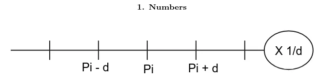
A Magnified View of the Hyperreal Line12 1. Numbers
X 1/d
Pi
Pi + d
Pi - d
Figure 1.1: Magnification at Pi
The basic fact is that finite numbers only differ from reals by an infinitesimal. (This is equivalent to Dedekind’s Completeness Axiom.)
Theorem 1.11.
Standard Parts of Finite NumbersEvery finite hyperreal number x differs from some ordinary real number r by an infinitesimal amount,x−r≈0orx≈r. The ordinary real number infinitely near xis called the standard part of x,r= st(x).
Proof:
Suppose x is a finite hyperreal. Define a cut in the real numbers by letting A be the set of all real numbers satisfying a≤xand lettingB be the set of all real numbersb with x < b. Both A and B are nonempty because x is finite. Everya in A is below every b in B by transitivity of the order on the hyperreals. The completeness of the real numbers means that there is a realrat the gap betweenA andB. We must havex≈r, because if x−r >1/m, say, thenr+ 1/(2m)< xand by the gap property would need to be inB.
A picture of the hyperreal number line looks like the ordinary real line at unit scale. We can’t draw far enough to get to the infinitely large part and this theorem says each finite number is indistinguishably close to a real number. If we magnify or compress by new number amounts we can see new structure.
You still cannot divide by zero (that violates rules of algebra), but if δ is a positive infinitesimal, we can compute the following:
−δ, δ2, 1
δ What can we say about these quantities?
The idealization of infinitesimals lets us have our cake and eat it too. Since δ6= 0, we can divide byδ. However, sinceδ is tiny, 1/δ must be HUGE.
Example 1.5.
Negative infinitesimalsIn ordinary algebra, if ∆>0, then−∆<0, so we can apply this rule to the infinitesimal numberδ and conclude that−δ <0, since δ >0.
Example 1.6.
Orders of infinitesimalsIn ordinary algebra, if 0<∆<1, then 0<∆2<∆, so 0< δ2< δ.
We want you to formulate this more exactly in the next exercise. Just assume δ is very small, but positive. Formulate what you want to draw algebraically. Try some small ordinary numbers as examples, like δ= 0.01. Plotδ at unit scale and place δ2 accurately
on the figure.
Small, Medium and Large Numbers 13
For real numbers if 0 <∆ <1/nthen n < 1/∆. Since δ is infinitesimal, 0< δ < 1/n for every natural number n = 1,2,3, . . . Using ordinary rules of algebra, but substituting the infinitesimal δ, we see that H = 1/δ > n is larger than any natural number n (or is “infinitely large”), that is, 1<2<3< . . . < n < H, for every natural numbern. We can “see” infinitely large numbers by turning the microscope around and looking in the other end.
The new algebraic rules are the ones that tell us when quantities are infinitely close, a≈b. Such rules, of course, do not follow from rules about ordinary high school numbers, but the rules are intuitive and simple. More important, they let us ‘calculate limits’ directly.
Theorem 1.12.
Computation Rules for Finite and Infinitesimal Numbers (a) Ifpandq are finite, so arep+qandp·q.(b) Ifε andδare infinitesimal, so isε+δ.
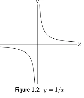
(c) Ifδ≈0andq is finite, then q·δ≈0. (finite x infsml = infsml) (d) 1/0 is still undefined and1/x is infinitely large only whenx≈0.
To understand these rules, just think of pand q as “fixed,” if large, andδ as being as small as you please (but not zero). It is not hard to give formal proofs from the definitions above, but this intuitive understanding is more important. The last rule can be “seen” on the graph ofy= 1/x. Look at the graph and move down near the valuesx≈0.
x
y
Figure 1.2: y= 1/x
Proof:
We prove rule (c) and leave the others to the exercises. If qis finite, there is a natural number mso that |q|< m. We want to show that |q·δ|<1/nfor any natural numbern. Sinceδis infinitesimal, we have|δ|<1/(n·m). By Exercise 1.2.5,|q| · |δ|< m·n·1m=
1
m.
Example 1.8.
y=x3⇒dy= 3x2 dx, for finitexThe error term in the increment off[x] =x3, computed above is
ε= (δx[3x+δx])
14 1. Numbers
justifies the local linearity ofx3at finite values ofx, that is, we have used the approximation
rules to show that
f[x+δx] =f[x] +f′[x]δx+ε δx
withε≈0 wheneverδx≈0 andxis finite, wheref[x] =x3 andf′[x] = 3x2.
Exercise set 1.4
1.
Draw the view of the ideal number line when viewed under an infinitesimal microscope of power 1/δ. Which number appears unit size? How big does δ2 appear at this scale?Where do the numbersδand δ3 appear on a plot of magnification1/δ2?
2.
Backwards microscopes or compressionDraw the view of the new number line when viewed under an infinitesimal microscope with its magnification reversed to powerδ(not1/δ). What size does the infinitely large numberH (HUGE) appear to be? What size does the finite (ordinary) numberm= 109
appear to be? Can you draw the numberH2 on the plot?
3.
y=xp⇒dy=p xp−1 dx,p= 1,2,3, . . .For eachf[x] =xp below:
(a) Compute f[x+δx]−f[x] and simplify, writing the increment equation: f[x+δx]−f[x] =f′[x]·δx+ε·δx
= [term inxbut not δx]δx+ [observed microscopic error]δx
Notice that we can solve the increment equation for ε= f[x+δx]−f[x]
δx −f
′[x]
(b) Show that ε≈0 ifδx≈0 and xis finite. Does xneed to be finite, or can it be any hyperreal number and still have ε≈0?
(1) If f[x] =x1, thenf′[x] = 1x0= 1 andε= 0.
(2) If f[x] =x2, thenf′[x] = 2xandε=δx.
(3) If f[x] =x3, thenf′[x] = 3x2 andε= (3x+δx)δx.
(4) If f[x] =x4, thenf′[x] = 4x3 andε= (6x2+ 4xδx+δx2)δx.
(5) If f[x] =x5, thenf′[x] = 5x4 andε= (10x3+ 10x2δx+ 5xδx2+δx3)δx.
4.
Exceptional Numbers and the Derivative ofy= 1 x (a) Let f[x] = 1/x and show thatf[x+δx]−f[x]
δx =
−1 x(x+δx) (b) Compute
ε= −1 x(x+δx)+
1 x2 =δx·
1 x2(x+δx)
(c) Show that this gives
f[x+δx]−f[x] =f′[x]·δx+ε·δx
when f′[x] =−1/x2.
Small, Medium and Large Numbers 15
5.
Exceptional Numbers and the Derivative ofy=√x (a) Let f[x] =√xand computef[x+δx]−f[x] = √ 1
x+δx+√x (b) Compute
ε=√ 1
x+δx+√x− 1 2√x =
−1
2√x(√x+δx+√x)2·δx
(c) Show that this gives
f[x+δx]−f[x] =f′[x]·δx+ε·δx when f′[x] = 1
2√x.
(d) Show that ε≈0 provided xis positive and NOT infinitesimal (and in particular is not zero.)
CHAPTER
2
Functional Identities
In high school you learned that trig functions satisfy certain iden-tities or that logarithms have certain “properties.” This chapter extends the idea of functional identities from specific cases to a defining property of an unknown function.
The use of “unknown functions” is of fundamental importance in calculus, and other branches of mathematics and science. For example, differential equations can be viewed as identities for unknown functions.
One reason that students sometimes have difficulty understanding the meaning of deriva-tives or even the general rules for finding derivaderiva-tives is that those things involve equations in unknown functions. The symbolic rules for differentiation and the increment approximation defining derivatives involve unknown functions. It is important for you to get used to this “higher type variable,” an unknown function. This chapter can form a bridge between the specific identities of high school and the unknown function variables from rules of calculus and differential equations.
2.1
Specific Functional Identities
All the the identities you need to recall from high school are:
(Cos[x])2+ (Sin[x])2= 1 CircleIden
Cos[x+y] = Cos[x] Cos[y]−Sin[x] Sin[y] CosSum Sin[x+y] = Sin[x] Cos[y] + Sin[y] Cos[x] SinSum
bx+y=bxby ExpSum
(bx)y =bx·y RepeatedExp
Log[x·y] = Log[x] + Log[y] LogProd
Log[xp] =pLog[x] LogPower
but you must be able to use these identities. Some practice exercises using these familiar identities are given in main text CD Chapter 28.
18 2. Functional Identities
2.2
General Functional Identities
A general functional identity is an equation which is satisfied by an unknown function (or a number of functions) over its domain.
The function
f[x] = 2x
satisfies f[x+y] = 2(x+y)= 2x2y =f[x]f[y], so eliminating the two middle terms, we see
that the functionf[x] = 2xsatisfies the functional identity
f[x+y] =f[x]f[y] (ExpSum)
It is important to pay attention to the variable or variables in a functional identity. In order for an equation involving a function to be a functional identity, the equation must be valid for allvalues of the variables in question. Equation (ExpSum) above is satisfied by the function f[x] = 2xfor allxandy. For the functionf[x] =x, it is true thatf[2 + 2] =f[2]f[2], but
f[3 + 1]6=f[3]f[1], so =xdoes not satisfy functional identity (ExpSum).
Functional identities are a sort of ‘higher laws of algebra.’ Observe the notational simi-larity between the distributive law for multiplication over addition,
m·(x+y) =m·x+m·y and the additive functional identity
f[x+y] =f[x] +f[y] (Additive)
Most functionsf[x] do not satisfy the additive identity. For example, 1
x+y 6= 1 x+
1
y and
√
x+y6=√x+√y
The fact that these are not identities means that forsomechoices ofxandyin the domains of the respective functions f[x] = 1/x and f[x] = √x, the two sides are not equal. You will show below that the only differentiable functions that do satisfy the additive functional identity are the functions f[x] =m·x. In other words, the additive functional identity is nearly equivalent to the distributive law; the only unknown (differentiable) function that satisfies it ismultiplication. Other functional identities such as the 7 given at the start of this chapter capture the most important features of the functions that satisfy the respective identities. For example, the pair of functionsf[x] = 1/x andg[x] =√xdo not satisfy the addition formula for the sine function, either.
Example 2.1.
The Microscope EquationThe “microscope equation” defining the differentiability of a functionf[x] (see Chapter 5 of the text),
General Functional Identities 19
with ε ≈ 0 if δx ≈ 0, is similar to a functional identity in that it involves an unknown function f[x] and its related unknown derivative function f′[x]. It “relates” the function
f[x] to its derivative dxdf =f′[x].
You should think of (Micro) as the definition of the derivative off[x] at a givenx, but also keep in mind that (Micro) is the definition of the derivative ofanyfunction. If we let f[x] vary over a number of different functions, we get different derivatives. The equation (Micro) can be viewed as an equation in which the function,f[x], is the variable input, and the output is the derivative dxdf.
To make this idea clearer, we rewrite (Micro) by solving for dxdf: ) df
dx =
f[x+δx]−f[x]
δx −ε
or df
dx = lim∆x→0
f[x+δx]−f[x] ∆x
If we plug in the “input” functionf[x] =x2into this equation, the output is df
dx = 2x. If we
plug in the “input” functionf[x] = Log[x], the output is dxdf = 1
x. The microscope equation
involves unknown functions, but strictly speaking, it is not a functional identity, because of the error term ε (or the limit which can be used to formalize the error). It is only an approximate identity.
Example 2.2.
Rules of DifferentiationThe various “differentiation rules,” the Superposition Rule, the Product Rule and the Chain Rule (from Chapter 6 of the text) are functional identities relating functions and their derivatives. For example, the Product Rule states:
d(f[x]g[x])
dx =
df
dxg[x] +f[x] dg dx
We can think off[x] andg[x] as “variables” which vary by simply choosing different actual functions forf[x] andg[x]. Then the Product Rule yields an identity between the choices off[x] andg[x], and their derivatives. For example, choosingf[x] =x2 andg[x] = Log[x]
and plugging into the Product Rule yields d(x2Log[x])
dx = 2xLog[x] +x
21
x
Choosingf[x] =x3 andg[x] = Exp[x] and plugging into the Product Rule yields
d(x3Exp[x])
dx = 3x
2Exp[x] +x3Exp[x]
If we choose f[x] = x5, but do not make a specific choice for g[x], plugging into the
Product Rule will yield
d(x5g[x])
dx = 5x
4g[x] +x5dg
dx
20 2. Functional Identities
Exercise set 2.2
1.
(a) Verify that for any positive number,b, the functionf[x] =bx satisfies thefunc-tional identity (ExpSum) above for all xandy.
(b) Is (ExpSum) valid (for all x and y) for the function f[x] = x2 or f[x] = x3?
Justify your answer.
2.
Define f[x] = Log[x] where xis any positive number. Why does this f[x] satisfy the functional identitiesf[x·y] =f[x] +f[y] (LogProd)
and
f[xk] =kf[x] (LogPower)
wherex,y, andkare variables. What restrictions should be placed onxandy for the above equations to be valid? What is the domain of the logarithm?
3.
Find values ofxand y so that the left and right sides of each of the additive formulas for 1/x and√xabove are not equal.4.
Show that1/xand√xalso do not satisfy the identity (SinSum), that is, 1x+y = 1 x
√y+√
x 1 y
is false for some choices ofxandy in the domains of these functions.
5.
(a) Suppose that f[x] is anunknown function which is known to satisfy (LogProd) (sof[x] behaves “like”Log[x], but we don’t know iff[x] isLog[x]), and suppose that f[0]is a well-defined number (even though we don’t specify exactly whatf[0] is). Show that this function f[x] must be the zero function, that is show that f[x] = 0for everyx. (Hint: Use the fact that0∗x= 0).(b) Suppose that f[x]is an unknown function which is known to satisfy (LogPower) for all x >0and allk. Show thatf[1]must equal0,f[1] = 0. (Hint: Fixx= 1, and try different values of k).
6.
(a) Let m andbbe fixed numbers and define f[x] =m x+bVerify that if b= 0, the above function satisfies the functional identity f[x] =x f[1]
(Mult)
for all xand that ifb6= 0,f[x] will not satisfy (Mult) for allx(that is, given a nonzerob, there will be at least onexfor which (Mult) is not true).
(b) Prove that any function satisfying (Mult) also automatically satisfies the two functional identities
f[x+y] =f[x] +f[y] (Additive)
and
f[x y] =x f[y] (Multiplicative)
The Function Extension Axiom 21
(c) Suppose f[x] is a function which satisfies (Mult) (and for now that is the only thing you know about f[x]). Prove thatf[x] must be of the form f[x] =m·x, for some fixed numberm (this is almost obvious).
(d) Prove that a general power function,f[x] =mxk wherekis a positve integer and
m is a fixed number, will not satisfy (Mult) for all xif k6= 1, (that is, ifk6= 1, there will be at least onexfor which (Mult) is not true).
(e) Prove that f[x] = Sin[x] does not satisfy the additive identity. (f) Prove that f[x] = 2xdoes not satisfy the additive identity.
7.
(a) Let f[x] and g[x] be unknown functions which are known to satisfy f[1] = 2,df
dx(1) = 3,g(1) =−3, dg
dx(1) = 4. Leth(x) =f[x]g[x]. Compute dh dx(1).
(b) Differentiate the general Product Rule identity to get a formula for d2(f g)
dx2
Use your rule to compute ddx2(h2)(1)if
d2(f)
dx2 (1) = 5and
d2(g)
dx2 (1) =−2, using other
values from part 1 of this exercise.
2.3
The Function Extension Axiom
This section shows that all real functions have hyperreal extensions that are “natural” from the point of view of properties of the original function.
Roughly speaking, the Function Extension Axiom for hyperreal numbers says that the natural extension of any real function obeys the same functional identities and inequalities as the original function. In Example 2.7, we use the identity,
f[x+δx] =f[x]·f[δx]
withxhyperreal andδx≈0 infinitesimal wheref[x] is a real function satisfyingf[x+y] = f[x]·f[y]. The reason this statement of the Function Extension Axiom is ‘rough’ is because we need to know precisely which values of the variables are permitted. Logically, we can express the axiom in a way that covers all cases at one time, but this is a little complicated so we will precede that statement with some important examples.
The Function Extension Axiom is stated so that we can apply it to the Log identity in the form of the implication
(x >0 &y >0)⇒Log[x] and Log[y] are defined and Log[x·y] = Log[x] + Log[y] The natural extension of Log[·] is defined for all positive hyperreals and its identities hold for hyperreal numbers satisfyingx >0 andy >0. The other identities hold for all hyperrealx andy. To make all such statements implications, we can state the exponential sum equation as
22 2. Functional Identities
The differential
d(Sin[θ]) = Cos[θ]dθ
is a notational summary of the valid approximation
Sin[θ+δθ]−Sin[θ] = Cos[θ]δθ+ε·δθ
where ε ≈ 0 whenδθ ≈ 0. The derivation of this approximation based on magnifying a circle (given in a CD Section of Chapter 5 of the text) can be made precise by using the Function Extension Axiom in the place where it locates (Cos[θ+δθ],Sin[θ+δθ]) on the unit circle. This is simply using the extension of the (CircleIden) identity to hyperreal numbers, (Cos[θ+δθ])2+ (Sin[θ+δθ])2= 1.
Logical Real Expressions, Formulas and Statements
Logical real expressions are built up from numbers and variables using functions. Here is the precise definition.
(a) A real number is a real expression.
(b) A variable standing alone is a real expression.
(c) IfE1, E2,· · ·, En are a real expressions andf[x1, x2,· · · , xn] is a real function ofn
variables, then f[E1, E2,· · · , En] is a real expression.
A logical real formula is one of the following:
(a) An equation between real expressions,E1=E2.
(b) An inequality between real expressions, E1< E2,E1 ≤E2,E1> E2, E1≥E2, or
E16=E2.
(c) A statement of the form “E is defined” or of the form “E is undefined.”
LetS andT be finite sets of real formulas. A logical real statement is an implication of the form,
S⇒T
or“whenever every formula inS is true, then every formula inT is true.”
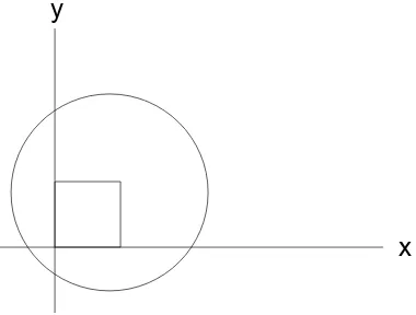
Logical real statements allow us to formalize statements like: “Every point in the square below lies in the circle below.” Formalizing the statement does not make it true or false. Consider the figure below.
x
y
The Function Extension Axiom 23
The inside of the square shown can be described formally as the set of points satisfying the equations in the setS={0≤x, 0≤y,x≤1.2,y≤1.2}. The inside of the circle shown can be defined as the set of points satisfying the single equationT ={(x−1)2+(y−1)2≤1.62}.
This is the circle of radius 1.6 centered at the point (1,1). The logical real statementS⇒T means that every point inside the square lies inside the circle. The statement is true for every real xand y. First of all, it is clear by visual inspection. Second, points (x, y) that make one or more of the formulas inS false produce a false premise, so no matter whether or not they lie in the circle, the implication is logically true (if uninteresting).
The logical real statement T ⇒ S is a valid logical statement, but it is false since it says every point inside the circle lies inside the square. Naturally, only true logical real statements transfer to the hyperreal numbers.
Axiom 2.1.
The Function Extension AxiomEvery logical real statement that holds for all real numbers also holds for all hyper-real numbers when the hyper-real functions in the statement are replaced by their natural extensions.
The Function Extension Axiom establishes the 5 identities for all hyperreal numbers, becausex=xandy=y always holds. Here is an example.
Example 2.3.
The Extended Addition Formula for SineS ={x=x, y=y} ⇒T ={Sin[x] is defined, Sin[y] is defined, Cos[x] is defined, Cos[y] is defined,
Sin[x+y] = Sin[x] Cos[y] + Sin[y] Cos[x]}
The informal interpretation of the extended identity is that the addition formula for sine holds for all hyperreals.
Example 2.4.
The Extended Formulas for LogWe may take S to be formulas x > 0, y > 0 and p = p and T to be the functional identities for the natural log plus the statements “Log[ ] is defined,” etc. The Function Extension Axiom establishes that log is defined for positive hyperreals and satisfies the two basic log identities for positive hyperreals.
Example 2.5.
Abstract Uses of Function ExtensionThere are two general uses of the Function Extension Axiom that underlie most of the theoretical problems in calculus. These involve extension of the discrete maximum and extension of finite summation. The proof of the Extreme Value Theorem 4.4 below uses a hyperfinite maximum, while the proof of the Fundamental Theorem of Integral Calculus 5.1 uses hyperfinite summation.
24 2. Functional Identities
Example 2.6.
The Increment ApproximationNote: The increment approximation
f[x+δx] =f[x] +f′[x]·δx+ε·δx withε≈0 forδx≈0 and the simpler statement
δx≈0 ⇒ f′[x]≈f[x] +δx)δx −f[x]
are notreallogical expressions, because they contain the relation≈, which is not included in the formation rules for logical real statements. (The relation≈does not apply to ordinary real numbers, except in the trivial casex=y.)
For example, ifθ is any hyperreal andδθ≈0, then
Sin[θ+δθ] = Sin[θ] Cos[δθ] + Sin[δθ] Cos[θ]
by the natural extension of the addition formula for sine above. Notice that the natural extension does NOT tell us the interesting and important estimate
Sin[θ+δθ] = Sin[θ] +δθ·Cos[θ] +ε·δθ
withε≈0 whenδθ≈0. (I.e., Cos[δθ] = 1 +ιδθ and Sin[δθ]/δθ≈1 are true, but not real logical statements we can derive just from natural extensions.)
Exercise set 2.3
1.
Write a formal logical real statement S ⇒T that says, “Every point inside the circle of radius 2, centered at(−1,3) lies outside the square with sides x= 0,y = 0,x= 1, y =−1. Draw a figure and decide whether or not this is a true statement for all real values of the variables.2.
Write a formal logical real statementS⇒T that is equivalent to each of the functional identities on the first page of the chapter and interpret the extended identities in the hyperreals.2.4
Additive Functions
Additive Functions 25
In the early 1800s, Cauchy asked the question: Must a function satisfying f[x+y] =f[x] +f[y]
(Additive)
be of the formf[x] =m·x? This was not solved until the late 1800s by Hamel. The answer is “No.” There are some very strange functions satisfying the additive identity that are not simple linear functions. However, these strange functions are not differentiable. We will solve a variant of Cauchy’s problem for differentiable functions.
Example 2.7.
A Variation on Cauchy’s ProblemSuppose an unknown differentiable function f[x] satisfies the (ExpSum) identity for all xand y,
f[x+y] =f[x]·f[y] Does the function have to bef[x] =bx for some positiveb?
Since our unknown function f[x] satisfies the (ExpSum) identity and is differentiable, both of the following equations must hold:
f[x+y] =f[x]·f[y]
f[x+δx] =f[x] +f′[x]·δx+ε·δx
We lety=δxin the first identity to compare it with the increment approximation, f[x+δx] =f[x]·f[δx]
f[x+δx] =f[x] +f′[x]·δx+ε·δx so
f[x]·f[δx] =f[x] +f′[x]·δx+ε·δx f[x][f[δx]−1] =f′[x]·δx+ε·δx f′[x] =f[x]f[δx]−1
δx −ε or
f′[x] f[x] =
f[δx]−1 δx −ε
with ε ≈ 0 whenδx ≈ 0. The identity still holds with hyperreal inputs by the Function Extension Axiom. Since the left side of the last equation depends only onxand the right hand side does not depend onxat all, we must have f[δxδx]−1≈k, a constant, or f[∆∆xx]−1 →k as ∆x→ 0. In other words, a differentiable function that satisfies the (ExpSum) identity satisfies the differential equation
df dx =k f
What is the value of our unknown function at zero,f[0]? For anyxandy= 0, we have f[x] =f[x+ 0] =f[x]·f[0]
so unlessf[x] = 0 for allx, we must havef[0] = 1.
26 2. Functional Identities
and
(2) how a quantity changes,
then you can compute subsequent values of the quantity. In this problem we have found (1)f[0] = 1 and (2) dxdf =k f. We can use this information with the computer to calculate values of our unknown functionf[x]. The unique symbolic solution to
f[0] = 1 df dx =k f is
f[x] =ek x The identity (Repeated Exp) allows us to write this as
f[x] =ek x= (ek)x=bx
where b =ek. In other words, we have shown that the only differentiable functions that
satisfy the (ExpSum) identity are the ones you know from high school,bx.
Problem 2.1.
Smooth Additive Functions ARE LinearH
Suppose an unknown function is additive and differentiable, so it satisfies both
f[x+δx] =f[x] +f[δx] (Additive)
and
f[x+δx] =f[x] +f′[x]·δx+ε·δx (Micro)
Solve these two equations for f′[x] and argue that since the right side of the equation does
not depend on x,f′[x] must be constant. (Or f[∆x]
∆x →f′[x1] and f[∆x]
∆x →f′[x2], but since
the left hand side is the same,f′[x
1] =f′[x2].)
What is the value off[0]if f[x] satisfies the additive identity?
The derivative of an unknown functionf[x]is constant and f[0] = 0, what can we say about the function? (Hint: Sketch its graph.)
N
A project explores this symbolic kind of ‘linearity’ and the microscope equation from another angle.
2.5
The Motion of a Pendulum
The Motion of a Pendulum 27
For example, suppose you know a functionθ[t] satisfies the differential equation d2θ
dt2 = Sin[θ[t]]
This equation arises in the study of the motion of a pendulum and θ[t] does not have a closed form expression. (Thereisno formula forθ[t].) Suppose you know θ[0] = π
2. Then
the differential equation forces d2θ
dt2[0] = Sin[θ[0]] = Sin[
π 2] = 1
We can also use the differential equation forθto get information about the higher deriva-tives of θ[t]. Say we know that dθdt[0] = 2. Differentiating both sides of the differential equation yields
d3θ
dt3 = Cos[θ[t]]
dθ dt
by the Chain Rule. Using the above information, we conclude that d3θ
dt3[0] = Cos[θ[0]]
dθ
dt[0] = Cos[ π 2]2 = 0
Problem 2.2.
H
Derive a formula for d4
θ
dt4 and prove that
d4
θ dt4[0] = 1.
-4
-2
2
4
w
-4
-2
2
4
x
Part 2
CHAPTER
3
The Theory of Limits
The intuitive notion of limit is that a quantity gets close to a “lim-iting” value as another quantity approaches a value. This chapter defines two important kinds of limits both with real numbers and with hyperreal numbers. The chapter also gives many computations of limits.
A basic fact about the sine function is
lim
x→0
Sin[x] x = 1
Notice that the limiting expression Sin[xx] is defined for 0<|x−0|<1, but not ifx= 0. The sine limit above is a difficult and interesting one. The important topic of this chapter is, “What does the limit expression mean?” Rather than the more “practical” question, “How do I compute a limit?”
Here is a simpler limit where we can see what is being approached.
lim
x→1
x2−1
x−1 = 2
While this limit expression is also only defined for 0 <|x−1|, or x6= 1, the mystery is easily resolved with a little algebra,
x2−1
x−1 =
(x−1)(x+ 1)
(x−1) =x+ 1
So,
lim
x→1
x2−1
x−1 = limx→1(x+ 1) = 2
The limit limx→1(x+ 1) = 2 is so obvious as to not need a technical definition. If xis
nearly 1, thenx+ 1 is nearly 1 + 1 = 2. So, while this simple example illustrates that the original expression does get closer and closer to 2 asxgets closer and closer to 1, it skirts the issue of “how close?”
32 3. The Theory of Limits
3.1
Plain Limits
Technically, there are two equivalent ways to define the simple continuous variable limit as follows.
Definition 3.1.
LimitLetf[x]be a real valued function defined for0<|x−a|<∆with∆a fixed positive real number. We say
lim
x→af[x] =b
when either of the equivalent the conditions of Theorem 3.2hold.
Theorem 3.2.
Limit of a Real VariableLetf[x]be a real valued function defined for0<|x−a|<∆with∆a fixed positive real number. Let b be a real number. Then the following are equivalent:
(a) Whenever the hyperreal number x satisfies 0 < |x−a| ≈ 0, the natural extension function satisfies
f[x]≈b
(b) For every accuracy toleranceθthere is a sufficiently small positive real num-berγ such that if the real number xsatisfies0<|x−a|< γ, then
|f[x]−b|< θ
Proof:
We show that (a) ⇒ (b) by proving that not (b) implies not (a), the contrapositive. Assume (b) fails. Then there is a realθ >0 such that for every realγ >0 there is a realx satisfying 0<|x−a|< γand |f[x]−b| ≥θ. LetX[γ] =xbe a real function that chooses such anxfor a particularγ. Then we have the equivalence
{γ >0} ⇔ {X[γ] is defined,0<|X[γ]−a|< γ,|f[X[γ]−b| ≥θ}
By the Function Extension Axiom 2.1 this equivalence holds for hyperreal numbers and the natural extensions of the real functions X[·] and f[·]. In particular, choose a positive infinitesimalγand apply the equivalence. We have 0<|X[γ]−a|< γand|f[X[γ]−b|> θ andθ is a positive real number. Hence,f[X[γ]] is not infinitely close tob, proving not (a) and completing the proof that (a) implies (b).
Conversely, suppose that (b) holds. Then for every positive realθ, there is a positive real γ such that 0<|x−a|< γ implies|f[x]−b|< θ. By the Function Extension Axiom 2.1, this implication holds for hyperreal numbers. Ifξ≈a, then 0<|ξ−a|< γfor every realγ, so|f[ξ]−b|< θfor every real positiveθ. In other words,f[ξ]≈b, showing that (b) implies (a) and completing the proof of the theorem.
Plain Limits 33
Suppose we wish to prove completely rigorously that lim
The intuitive limit computation of just setting ∆x= 0 is one way to “see” the answer, lim
but this certainly does not demonstrate the “epsilon - delta” condition (b).
Condition (a) is almost as easy to establish as the intuitive limit computation. We wish to show that whenδx≈0
1 2(2 +δx) ≈
1 4 Subtract and do some algebra,
1
We complete the proof using the computation rules of Theorem 1.12. The fraction−1/(4(2+ δx)) is finite because 4(2 +δx)≈8 is not infinitesimal. The infinitesimal δxtimes a finite number is infinitesimal.
This is a complete rigorous proof of the limit. Theorem 3.2 shows that the “epsilon - delta” condition (b) holds.
Exercise set 3.1
1.
Prove rigorously that the limitlim∆x→03(3+∆1 x)= 19. Use your choice of condition (a)or condition (b) from Theorem3.2.
2.
Prove rigorously that the limit lim∆x→0√4+∆1x+√4 = 14. Use your choice of condition(a) or condition (b) from Theorem 3.2.
3.
The limitlimx→0Sin[xx] = 1means that sine of a small value is nearly equal to the value,and near in a strong sense. Suppose the natural extension of a function f[x] satisfies f[ξ] ≈0 whenever ξ ≈ 0. Does this mean that limx→0f[xx] exists? (HINT: What is
limx→0√x? What is√ξ/ξ?)
4.
Assume that the derivative of sine is cosine and use the increment approximation34 3. The Theory of Limits
withε≈0 when δx≈0, to prove the limitlimx→0Sin[xx] = 1. (It means essentially the
same thing as the derivative of sine at zero is 1. HINT: Take x= 0 andδx=xin the increment approximation.)
3.2
Function Limits
Many limits in calculus are limits of functions. For example, the derivative is a limit and the derivative of x3 is the limit function 3x2. This section
defines the function limits used in differentiation theory.
Example 3.2.
A Function LimitThe derivative ofx3is 3x2, a function. When we compute the derivative we use the limit
lim
∆x→0
(x+ ∆x)3−x3
∆x
Again, the limiting expression is undefined at ∆x= 0. Algebra makes the limit intuitively clear,
(x+ ∆x)3−x3
∆x =
(x3+ 3x2∆x+ 3x∆x2+ ∆x3)−x3
∆x = 3x
2+ 3x∆x+ ∆x2
The terms with ∆xtend to zero as ∆xtends to zero.
lim
∆x→0
(x+ ∆x)3−x3
∆x = lim∆x→0(3x
2+ 3x∆x+ ∆x2) = 3x2
This is clear without a lot of elaborate estimation, but there is an important point that might be missed if you don’t remember that you are taking the limit of a function. The graph of the approximating function approaches the graph of the derivative function. This more powerful approximation (than that just a particular value of x) makes much of the theory of calculus clearer and more intuitive than a fixedx approach. Intuitively, it is no harder than the fixedxapproach and infinitesimals give us a way to establish the “uniform” tolerances with computations almost like the intuitive approach.
Definition 3.3.
Locally Uniform Function LimitLet f[x]andF[x,∆x] be real valued functions defined whenxis in a real interval (a, b)and0<∆x <∆with ∆ a fixed positive real number. We say
lim
∆x→0F[x,∆x] =f[x]
Function Limits 35
Theorem 3.4.
Limit of a Real FunctionLet f[x]andF[x,∆x] be real valued functions defined whenxis in a real interval (a, b)and0<∆x <∆ with∆a fixed positive real number. Then the following are equivalent:
(a) Whenever the hyperreal numbers δxand xsatisfy 0<|δx| ≈0,xis finite, anda < x < bwith neitherx≈anorx≈b, the natural extension functions satisfy
F[x, δx]≈f[x]
(b) For every accuracy tolerance θ and every real α and β in (a, b), there is a sufficiently small positive real numberγ such that if the real number ∆x satisfies0<|∆x|< γand the real number xsatisfiesα≤x≤β, then
|F[x,∆x]−f[x]|< θ
Proof:
First, we prove not (b) implies not (a). If (b) fails, there are realαandβ,a < α < β < b, and real positiveθ such that for every real positiveγthere arexand ∆xsatisfying
0<∆x < γ, α≤x≤β, |F[x,∆x]−f[x]| ≥θ Define real functionsX[γ] andDX[γ] that select such values of xand ∆x,
0< DX[γ]< γ, α≤X[γ]≤β, |F[X[γ], DX[γ]]−f[X[γ]]| ≥θ Now apply the Function Extension Axiom 2.1 to the equivalent sets of inequalities,
{γ >0} ⇔ {0< DX[γ]< γ, α≤X[γ]≤β, |F[X[γ], DX[γ]]−f[X[γ]]| ≥θ}
Choose an infinitesimalγ≈0 and letx=X[γ] andδx=DX[γ]. Then 0< δx < γ≈0, α≤x≤β, |F[x, δx]−f[x]| ≥θ
soF[x, δx]−f[x] is not infinitesimal showing not (a) holds and proving (a) implies (b). Now we prove that (b) implies (a). Letδxbe a non zero infinitesimal and let xsatisfy the conditions of (a). We show thatF[x, δx]≈f[x] by showing that for any positive realθ,
|F[x, δx]−f[x]|< θ. Fix any one such value ofθ.
Sincexis finite and not infinitely neara norb, there are real valuesαand β satisfying a < α < β < b. Apply condition (b) to theseα andβ together withθ fixed above. Then there is a positive real γ so that for every real ξ and ∆x satisfying 0 < |∆x| < γ and α≤ξ≤β, we have|F[ξ,∆x]−f[ξ]|< θ. In other words, the following implication holds in the real numbers,
{0<|∆x|< γ, α≤ξ≤β} ⇒ {|F[ξ,∆x]−f[ξ]|< θ}
Apply the Function Extension Axiom 2.1 to see that the same implication holds in the hyperreals. Moreover,x = ξ and nonzero ∆x= δx ≈ 0 satisfy the left hand side of the implication, so the right side holds. Sinceθ was arbitrary, condition (a) is proved.
36 3. The Theory of Limits
The following limit is uniform on compact subintervals of (−∞,∞).
lim
∆x→0
(x+ ∆x)3−x3
∆x = lim∆x→0(3x
2+ 3x∆x+ ∆x2) = 3x2
A complete rigorous proof based on condition (a) can be obtained with the computation rules of Theorem 1.12. The difference is infinitesimal
(3x2+ 3x δx+δx2)−3x2= (3x+δx)δx
whenδxis infinitesimal. First, 3x+δxis finite because a sum of finite numbers is finite. Sec-ond, infinitesimal times finite is infinitesimal. This is a complete proof and by Theorem 3.4 shows that both conditions (b) and (c) also hold.
Exercise set 3.2
1.
Prove rigorously that the locally uniform function limit lim∆x→0x(x+∆1 x) = x12. Useyour choice of condition (a) or condition (b) from Theorem3.4.
2.
Prove rigorously that the locally uniform function limit lim∆x→0√x+∆1x+√x = 2√1x.Use your choice of condition (a), condition (b), or condition (c) from Theorem3.4.
3.
Prove the following:Theorem 3.5.
Locally Uniform DerivativesLet f[x] andf′[x] be real valued functions defined whenxis in a real interval
(a, b). Then the following are equivalent:
(a) Whenever the hyperreal numbers δx and xsatisfy δx≈ 0, x is finite, and a < x < b with neither x ≈ a nor x ≈ b, the natural extension functions satisfy
f[x+δx]−f[x] =f′[x]·δx+ε·δx
for ε≈0.
(b) For every accuracy toleranceθand every realαandβ in(a, b), there is a sufficiently small positive real numberγ such that if the real number ∆x satisfies0 <|∆x| < γ and the real numberx satisfiesα≤x≤β,
then
f[x+ ∆x]−f[x]
∆x −f
′[x]
< θ
(c) For every realcin (a, b), lim
x→c,∆x→0
f[x+ ∆x]−f[x]
∆x =f
′[c]
![Figure 5.1: y = f[x]](https://thumb-ap.123doks.com/thumbv2/123dok/2839696.1691842/65.612.128.476.282.450/figure-y-f-x.webp)
![Figure 5.2: Small View of x = g[y] and y = f[x] at (x0, y0)](https://thumb-ap.123doks.com/thumbv2/123dok/2839696.1691842/67.612.229.379.110.280/figure-small-view-x-g-y-y-f.webp)
![Figure 5.3: Small View of y = f[x] at (x0, y0)](https://thumb-ap.123doks.com/thumbv2/123dok/2839696.1691842/69.612.227.380.445.609/figure-small-view-y-f-x-x-y.webp)