Delivered by Ingenta to:
Guest User
IP : 222.124.194.25
Sun, 02 Oct 2011 10:05:30
Copyright © 2011 American Scientific Publishers All rights reserved
Printed in the United States of America
Advanced Science Letters
Vol. 4, 2807–2811, 2011
CFD Analysis for Merdeka 2 Solar Vehicle
Zahari Taha1, Rossi Passarella25∗
, Sugiyono3, Nasrudin Abd Rahim2, Jamali Md Sah4, and Aznijar Ahmad-Yazid2
1Faculty of Manufacturing Engineering and Technology Management, Universiti Malaysia Pahang, 26300, Malaysia 2Faculty of Engineering, University of Malaya, Kuala Lumpur, 50603, Malaysia
3Department of Mechanical and Industrial Engineering, Gadjah Mada University, Yogyakarta, 55281, Indonesia 4School of Manufacturing Engineering, Universiti Malaysia Perlis, 02600, Malaysia
5Department of Computer Engineering, University of Sriwijaya, Palembang, 30662, Indonesia
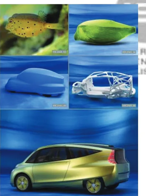
Vehicle’s low drag force is critical to achieve higher speed and for efficient energy usage. Most solar vehicles that participated in the World Solar Challenge event adopted the ‘cockroach’ shape which has been considered as the best shape to achieve optimum speed and aerodynamics characteristics. However, the team from University of Malaya decided to design their entry vehicle based on the profile of a box fish, said to possess an even lower drag coefficient value. This paper describes the aerodynamics characteristics numerical study of the solar vehicle using a computational fluid dynamics (CFD) code called FLUENT. The numerical computation is based on the frontal area of the vehicle and the obtained results have shown reasonable values of drag and lift coefficients when compared to ordinary road vehicles.
Keywords: Solar Vehicle, World Solar Challenge, Box Fish Shape, CFD.
1. INTRODUCTION
In 2009, the Center for Product Design and Manufacturing (CPDM) University of Malaya again participated in the World Solar Challenge (WSC) event with a second version of solar vehi-cle, named Merdeka 2; shown in Figure 1. The concept of using off-the-shelf components previously adopted for the first entrant in 2007, Merdeka was maintained. The Merdeka 2 was designed to be as similar possible to an ordinary vehicle except for the presence of solar panels at the roof of the vehicle. The vehi-cle main body structure was fabricated using aluminium alloy. The solar vehicle used a 48 V permanent magnet DC motor rotating at 3000 r.p.m. maximum. 4 units of 12 V deep cycle batteries were used to store the generated electrical energy from the photovoltaic solar panels, which in turn powered the motor. Each of the 12 V batteries were individually charged by sep-arate solar panels. 4 units of Maximum Power Point Tracking (MPPT) acted as the solar panels charging controller. During the 2009 event, with the average speed of 45 km/h, Merdeka 2 managed to finish 590 km of the approximately 3020 km, the total race distance. This achievement is approximately a 100% improvement compared to the performance of the previous entrant, Merdeka. The total manufacturing cost was approxi-mated at RM 50,000.00 (US$ 15,000). In the future, with lim-ited funding, it is foreseen that the researchers at CPDM will face a huge task to continue developing of the next solar vehicle
∗
Author to whom correspondence should be addressed.
with the aim of completing the race, or to overhaul Merdeka 2 achievement.
2. AERODYNAMICS ANALYSIS
Initially, the design concept for Merdeka 2 was based on the profile of the box fish, similar to the Mercedes Benz minivan, shown in Figure 2. This shape is said to possess a low drag coefficient value, Cd, of approximately 0.06, that can lead to a 20% reduction of fuel consumption.
To analyze the aerodynamics of the solar vehicle, a numer-ical method using computational fluid dynamics (CFD) code called FLUENT2 was performed. Generally, there are two steps
involved when performing this, firstly preparing the computa-tional domain and then conducting the numerical analysis. The first step, preparing the computational domain was carried out using Gambit, an integrated pre-processor of FLUENT to cre-ate the geometry of the model, generating the grid system and assigning the boundary conditions. The second step was car-ried out using the FLUENT processor, where the numerical model was set up and the computation performed to achieve the solution.
Delivered by Ingenta to:
Guest User
IP : 222.124.194.25
Sun, 02 Oct 2011 10:05:30
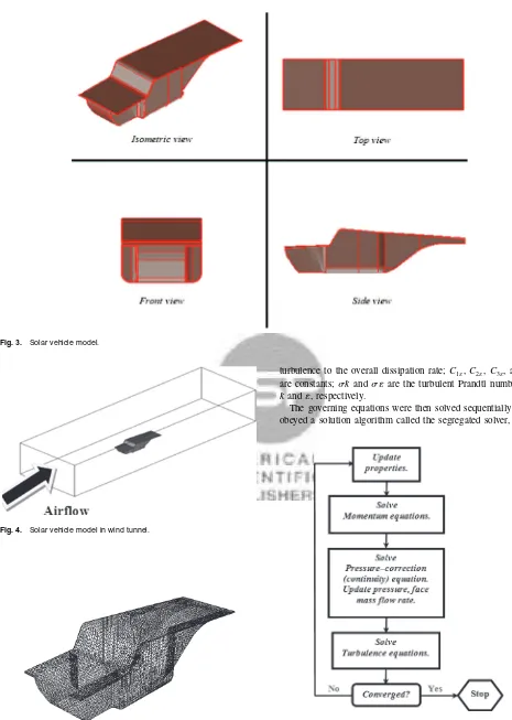
To perform the aerodynamic analysis in FLUENT, the model of the solar vehicle was drawn as if it is at the center of a wind tunnel with air being drawn across the model. This is shown in Figure 4. The model is also positioned 140 mm above of the wind tunnel base, following the lowest floor position of the solar vehi-cle above the road. The wind tunnel dimension was 23290 mm long, 6975 mm wide, and 4792 mm high. For the boundary con-ditions, the velocity-inlet and the pressure outlet were used on the upstream and the downstream boundaries, respectively. The non-slip conditions were applied on the entire solar vehicle sur-faces and on the walls of the wind tunnel.
The 3-D computational domain was then meshed using a hybrid meshing scheme which is a combination of hexahe-dral, tetrahedral and pyramidal grids. The total number of grids
Fig. 2. The Mercedes Benz minivan based on the boxfish profile.
Dui
The “Reynolds stresses” on the right-hand-side of Eq. (2) rep-resents the effects of turbulence which must be modeled. A com-monly employed method is the use of Boussinesq hypothesis to relate the Reynolds stresses to the mean velocity gradients, which is
Furthermore, additional transport equations were introduced in order to achieve “closure” Closure implies that there exist a sufficient number of equations to solve all the unknowns.
For this simulation, the turbulence is modeled using the Stan-dard k- model, as prescribe by Lauder and Spalding.3 There
are two additional transport equations that need to be solved; which are the turbulent kinetic energy (k and the turbulence dissipation rate (). Both the variables of k and were then used to compute the turbulent viscosity (t). Additionally, FLU-ENT documentation recommended that the non-equilibrium wall functions were employed for near-wall modeling by consider-ing their ability to deal with complex flows involvconsider-ing separation, re-attachment, other non-equilibrium effects and strong pressure gradients.2
The turbulent kinetic energy (kand the turbulence dissipation rate () were obtained from the following transport equations:
Dk The turbulent viscosity was computed as follows:
t=C
k2
(6)
In these equations,Gk represents the generation of turbulent
kinetic energy due to the mean velocity gradients;Gbis the
gen-eration of turbulent kinetic energy due to buoyancy; YM
Delivered by Ingenta to:
Guest User
IP : 222.124.194.25
Sun, 02 Oct 2011 10:05:30
Fig. 3. Solar vehicle model.
Fig. 4. Solar vehicle model in wind tunnel.
Fig. 5. Grids on surface of solar vehicle model.
turbulence to the overall dissipation rate;C1,C2,C3, andC are constants; kand are the turbulent Prandtl numbers for
kand, respectively.
The governing equations were then solved sequentially which obeyed a solution algorithm called the segregated solver, shown
Delivered by Ingenta to:
Guest User
IP : 222.124.194.25
Sun, 02 Oct 2011 10:05:30
discretization schemes used are as follows: a standard scheme for the pressure; the SIMPLE algorithm for the pressure-velocity coupling; and the second-order accurate upwind scheme for the momentum, turbulent kinetic energy (kand turbulence dissipa-tion rate (). Furthermore, several iterations of the solution loop must be performed before a converged solution was obtained.
The calculation was carried out under steady flow condition at the inlet velocity value of 60 km/h, and the flow was mod-eled as incompressible. During the solution process, the default under-relaxation factors, shown in Table I were selected to con-trol the update of computed variables, which was found to be
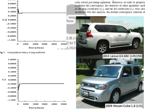
Fig. 7. Computational history of drag coefficient.
Fig. 8. Computational history of lift coefficient.
Fig. 9. Historical trend for drag coefficients of automobiles. Reprinted with permission from [4], Society of automotive engineers and SAE international congress and exposition, Vehicle aerodynamics: wake flows, computational fluid dynamics, and aerodynamic testing, Society of Automotive Engineers, Warrendale, PA(1992). © 1992.
near optimal for a large number of cases. The convergence of solution was monitored by checking the residuals of the numeri-cally solved governing equations. Moreover, in order to properly scrutinize the convergence, the behavior of other quantities such as the drag coefficient (Cdand the lift coefficient (Clwere also
monitored. For this analysis, the default convergence criterion of
Delivered by Ingenta to:
Guest User
IP : 222.124.194.25
Sun, 02 Oct 2011 10:05:30
Fig. 11. Effect of bottom rear upsweep angle on drag and down-ward lift coefficients.
Fig. 12. Velocity contour of the airflow around the solar vehicle (m/s).
each residual was reduced to allow the monitored quantities to stagnate at consistent values.
3. SIMULATION RESULTS AND VALIDATION
Figures 7 and 8 show the computational history of drag and lift coefficients. The calculations are based on the frontal area of the solar vehicle. The consistent, converged value for drag coefficient was 0.35, while it was-0.19 for lift coefficient.
When compared with the drag coefficient values reflected by the historical drag coefficient automobile, shown in Figure 9 and with a couple of existing vehicle in the market, shown in Figure 10, the drag coefficient value obtained from the simulation seemed reasonable and commendable.
Furthermore, the designed Merdeka 2, with no upsweep angle exhibited a lift coefficient value of−0.19 (equal to downward force coefficient value of 0.19) which was also acceptable when compared to Bearman et al. findings, reproduced in Figure 11.6
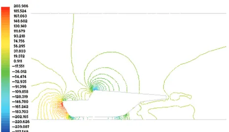
Figure 12 shows the velocity contour of the airflow around the solar vehicle. It can be observed that low velocities existed at the front of the solar vehicle. This can be attributed to the stagnation condition of air flow at that location. Figure 13 confirmed this
Fig. 13. Static pressure contour of the airflow around the solar vehicle (Pa).
observation by showing the highest static pressure noted at the front of the solar vehicle. Low velocities were also noted at the rear of the solar vehicle and at the front of the driver wind shield. These can be attributed to the formation of wake which created flow separation at those areas.
TheCd value obtained from the simulation was validated with
experimental results conducted in Australia and was reported by Taha et al.7 This comparison was performed based on power
consumption. The report indicated very slight difference in the theoretically calculated power at the speeds of 25, 36, and 60.7 km/h when compared with experimental values achieved. However there was no major difference at the maximum speed of 66.8 km/h.
4. CONCLUSION
Originally, the solar vehicle was designed based on the box fish shape. However, due to limited budget constrain and the require-ment to adopt current off-the-shelf components used for the fab-rication, the final Merdeka 2 shape was slightly different. The CFD analysis work of the Merdeka 2 solar vehicle was pre-sented, with the simulation achieving the values ofCd andCl at
0.35 and−0.19, respectively. There was also very slight differ-ence between the simulated results obtained through FLUENT computation when compared with the experimental data.
References and Notes
1. Mercedes-Benz bionic car modeled on boxfish. [Image on the Inter-net][updated 2005 June 7; Cited (2010) April 13] Available from: http://www.dancewithshadows.com/auto/mercedes-benz-bionic-car-gallery.asp.
2. Fluent, Fluent 6.3 User’s Guide, Fluent Inc.: Lebanon, NH(2006). 3. B. E. Launder and D. B. Spalding, Lectures in Mathematical Models of
Turbu-lence, Academic Press London, England(1972).
4. Society of automotive engineers and SAE international congress and expo-sition, Vehicle aerodynamics: wake flows, computational fluid dynamics, and aerodynamic testing, Society of Automotive Engineers, Warrendale, PA (1992).
5. Automobile drag Coefficients: WIKI.[Internet][Cited:(2010)April 15] Available from: http://wapedia.mobi/en/Automobile_drag_coefficients.
6. P. W. Bearman, D. D. Beer, E. Hamidy, and J. K. Harveyl, Society of Automo-tive Engineers Paper No. 880245(1988)Intl’ SAE Congress and Exposition, February-March. Detroit.
7. Z. Taha, R. Passarella, N. A. Rahim, J. Md Sah,ARPN J. Engineering and Applied Sciences5, 1(2010).