AUTOMATIC BUILDING ABSTRACTION FROM AERIAL PHOTOGRAMMETRY
Andreas Ley, Ronny H¨ansch∗
, Olaf Hellwich
Dept. of Computer Vision & Remote Sensing, Technische Universit¨at Berlin, Berlin -{andreas.ley, r.haensch, olaf.hellwich}@tu-berlin.de
KEY WORDS:Aerial imagery, photogrammetry, 3D reconstruction, abstraction
ABSTRACT:
Multi-view stereo has been shown to be a viable tool for the creation of realistic 3D city models. Nevertheless, it still states significant challenges since it results in dense, but noisy and incomplete point clouds when applied to aerial images. 3D city modelling usually requires a different representation of the 3D scene than these point clouds. This paper applies a fully-automatic pipeline to generate a simplified mesh from a given dense point cloud. The mesh provides a certain level of abstraction as it only consists of relatively large planar and textured surfaces. Thus, it is possible to remove noise, outlier, as well as clutter, while maintaining a high level of accuracy.
1. INTRODUCTION
The areas of photogrammetry and image-based 3D reconstruction have matured over the last decade. Nowadays, powerful methods and tools are at general disposal which allow to obtain impres-sive reconstructions of small-scale objects as well as of large-scale scenes. Despite the ongoing research on Structure-from-Motion (SfM) and Multi-View Stereo (MVS), more and more work is concerned with the further processing and analysis of the resulting point clouds. Typical examples include noise reduction, outlier removal, increasing the completeness by the use of prior knowledge, segmentation, semantic annotation, and simplifica-tion. Many applications that make use of digital 3D models do neither require nor desire raw point clouds or surface meshes with a large number of polygons. Instead, simple representations are needed that nonetheless give a realistic impression and provide a certain level of accuracy despite being a simplified and abstract version of the underlying 3D geometry.
One such application is the creation of realistic 3D models of ur-ban environments, which are used for urur-ban planning, city growth management, virtual tourist guides, etc. In particular web-based applications such as Google Earth led to an increased need of methods to create realistic 3D models of whole cities. Image-based 3D reconstruction has been favourably used due to its rel-atively low cost and ease of use. Furthermore, it is able to pro-vide dense, accurate, and textured 3D models. The applicational circumstances of such methods request procedures that are fully-automatic as well as efficient. Any kind of human interaction or the need of extensive processing would render the repetitive creation of large models infeasible. Furthermore, corresponding methods need to be flexible. Building shapes and other urban structures vary considerably within a single city and among dif-ferent cities of the world. Methods that rely on strong assump-tions about e.g. rectangular footprints will inevitably fail to de-liver accurate results. On the other hand, such methods need to be robust. MVS methods for 3D city modelling have to face weakly textured areas, strong occlusions, repetitive structures, reflective surfaces (e.g. glass elements on building facades), shadows and other non-stationary processes (e.g. moving objects), as well as strongly skewed views of certain scene elements (i.e. building facades). Consequently, the resulting point clouds are of lower quality than small-scale 3D reconstructions of near-range objects.
∗Corresponding author
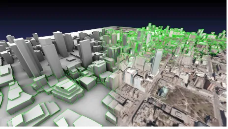
Figure 1. This paper applies a fully-automatic pipeline to obtain a simplified mesh from a given dense point cloud. The data shown in the figure is part of the evaluation dataset discussed in
Section 4.
They are noisy and contain partially unknown or distorted infor-mation. Nevertheless, visually pleasing and physically plausible models should be obtained in all cases despite input data of vary-ing quality. Furthermore, neither the raw dense point cloud even if with filled holes and cleaned from outliers nor a dense poly-gon mesh is desired for typical applications of 3D city modelling. Usually a certain level of abstraction is desired and needed to ob-tain models with as little noise as possible, without any clutter, and without the presence of irrelevant details.
In this paper a fully automatic pipeline is used to obtain a simpli-fied mesh from a given dense point cloud (see Figure 1). Strong assumptions about the data lead to priors that allow to rigorously remove noise and outliers on the one hand and introduce a certain level of abstraction on the other hand. Height maps are used as an intermediate step and interpreted as Markov Random Fields. This probabilistic optimization casts the surface reconstruction as a labelling problem and allows the inclusion of aforementioned priors (among other possibilities).
a) b) c) d) e) f)
Figure 2. An overview of the geometric processing steps of the applied pipeline: Starting from a point cloud (a), the ground plane and corresponding coordinate system is found (b). Next, a height map of discreet height values is estimated (c). The boundaries of this height map are simplified (d) and a constrained Delaunay triangulation is used on the horizontal surfaces (e). Finally, the horizontal
faces are displaced and the vertical faces are added (f).
2. RELATED WORK
Very good reconstruction results have been achieved for subur-ban areas by feature based approaches such as (Baillard and Zis-serman, 1999, Bignone et al., 1996, Fischer et al., 1999, Tail-landier and Deriche, 2004, Vosselman, 1999). However, these early methods rely on sparse line features to encode the whole building geometry. Since the fusion of such sparse features is error prone and unstable, the additional usage of other informa-tion sources such as cadastral maps has been addressed e.g. in (Baillard, 2004, Haala and Anders, 1996, Suveg and Vosselman, 2004). While this external data decreased the number of ambigui-ties, mismatches, and missing features during the fusion process, it cannot be assumed to be available for every (part of a) city. Even if it is available, it is of varying accuracy and need to be carefully aligned with the image data.
The use of height measurements, either obtained by laser scans or MVS, has been addressed before as well, e.g. in (Haala and Brenner, 1997, Maas and Vosselman, 1999). The works in (Sohn and Dowman, 2007, Chen et al., 2004, Hui et al., 2003, Zebedin et al., 2008) combine height information from a LIDAR scan with satellite images on the basis of line features. Our work differs by working on point clouds only, which can be generated with any sufficiently accurate MVS approach, and does not rely on the de-tection of any other sparse image features. It does not require any manual interaction and allows the generation of different levels of geometric detail.
An extensive amount of work has been published on the recon-struction of man made structures. Many of these methods use Markov Random Fields (MRFs), as for example (Furukawa et al., 2009a, Sinha et al., 2009) which compute a dense depth map and cast the reconstruction as a labelling problem. Each label designates a plane aligned with the main directions in man made structures (Furukawa et al., 2009a) or computed from line inter-sections (Sinha et al., 2009).
A subset of possible applications is the reconstruction of building facades from street-level imagery (in contrast to whole building models from aerial images). Corresponding methods range from rather simple approaches such as ruled vertical surfaces (Cornelis et al., 2007) to more sophisticated works with axis-aligned and facade-parallel rectangles (Xiao et al., 2009). The work in (Ley and Hellwich, 2016) uses an orthographic depth map as in (Xiao et al., 2009), but allows more general shapes during the regular-ization. It applies the MRF formulation directly in the coordinate system of the facade and constrains planes to be parallel to it.
Our work is heavily inspired by (Ley and Hellwich, 2016) and exploits the same processing chain to reconstruct building mod-els from aerial images instead of single facades from close-range imagery.
There are approaches available that extend depth maps to full 3D models having significantly more degrees of freedom, e.g.
(Fu-rukawa et al., 2009b, Chauve et al., 2010). However, similar to (Ley and Hellwich, 2016), a 2.5D approach is sufficient for the case of simple building models and states an optimization task that is easier to solve.
3. METHODOLOGY
Our approach follows closely the work in (Ley and Hellwich, 2016) and is described in the following subsections. The main difference is that the approach of (Ley and Hellwich, 2016), in order to reconstruct single building facades, operates in a coordi-nate system that is aligned to the facade plane while we apply this approach aligned to the ground plane to reconstruct entire cities. Figure 2 highlights the major steps.
Any standard SfM and MVS methods can be used as long as they are able to produce point clouds of sufficient quality. It should be noted that the proposed approach is not necessarily limited to a photogrammetric generation of the point cloud but could also exploit e.g. LIDAR data with the only difference that the resulting mesh would not be textured.
Although our goal is to produce a (simplistic) mesh as the 3D city model, height maps are estimated as an intermediate step. The usage of height maps has the important consequence that the general orientation of the ground plane needs to be accurately estimated. This is discussed in Section 3.1.
In a second step the individual values of the height map are es-timated. To this end, a set of height hypotheses is generated as described in Section 3.2 and subsequently used as labels for the pixels of the height map. In this way the estimation of continuous height values is cast as a discrete labelling problem which can be efficiently solved via energy minimization techniques.
To obtain a mesh from the estimated height map, the bound-aries of areas with homogeneous height values are detected and used for a constrained Delaunay triangulation as described in Section 3.3. In a last step the input images are used to compute a texture map (see Section 3.4).
3.1 Plane Alignment
kernels on the points’ 3D position and color value. The model fitting phase adjusts the plane parameters in order to fit them to the assigned data points.
Similar to (Ley and Hellwich, 2016), we use PEaRL with 30 hy-potheses, one of which is a clutter hypothesis to soak up outliers. Of the 29 plane hypotheses with differing support (i.e. number of assigned points), the one with the most support is selected as the ground plane. Since roofs etc. result in less points than the ground, the estimated ground plane usually describes the ground surface very well.
In a last step LSD line segments (Grompone von Gioi et al., 2012) are detected in the input images and projected onto the above established ground plane. A histogram of line directions provides the orientation of the main directions within the city. Of these one is selected to rotate the coordinate system of the ground plane accordingly. This ensures that the grid structure of the height map is properly aligned with most line structures in the scene, which is beneficial for planned cities.
3.2 Height Map
We assume that the ground surface of the city is mostly flat and can be covered by a plane. In case of non-flat city grounds a DSM could be used to account for the corresponding height vari-ations. Based on this assumption the remaining geometry of the city can be described by a 2.5D model, i.e. as a height map. Sur-faces parallel to the ground plane are mostly well visible in aerial images and are thus often well reconstructed in the point cloud. Surfaces perpendicular to the ground plane (such as facades) are often only visible in a few images under large skew and are thus often not well reconstructed. While the former ones are explic-itly modelled by the above mentioned 2.5D model, the later case is modelled only implicitly as height jumps in the map.
The height map is embedded into the coordinate system of the ground plane. It is extended in both coordinate directions such that it covers 98% of the input point cloud.
On the one hand, the estimation of the corresponding height val-ues is based on the input point cloud. On the other hand, it should be constrained by regularizations to overcome noise, outliers, and missing data. Ignoring non-flat roofs, many structures in a city are either parallel or perpendicular to the ground plane. A rea-sonable regularization is thus to enforce rectangular regions of equal height values as in (Ikehata et al., 2015, Xiao et al., 2009). However, this is too restrictive in our case as many buildings in a city cannot properly be described by rectangular outlines.
The work in (Ley and Hellwich, 2016) follows the pixel labelling approach in (Furukawa et al., 2009a, Sinha et al., 2009) which allows more general shapes. The point cloud data is projected onto the ground-aligned coordinate system in order to compute a histogram of height values. The maxima of this histogram pro-vide a set of height hypotheses, that represent possible “labels” which can be assigned to the pixels of the height map. This la-belling task is solved by interpreting the height map as a Markov Random Field (Ley and Hellwich, 2016) and minimizing the en-ergy term in Equation (1) through repeated graph cuts with alpha expansion (Boykov et al., 2001).
E=X p
Ed(hp) + X p,q∈N(p)
Es(hp, hq) (1)
The data termEd(hp)is the cost for assigning hypothesishp to height map pixel p. The binary term Es(hp, hq) enforces smoothness by penalizing the assignment of differing height hy-potheseshp, hqto neighboring pixelsp, q.
The data termEd(hp)is based on two individual factors: First, the clamped absolute difference between the height hypothesis
hp and the point cloud points projected into pixelp. Second, the number of free space votes that encode the condition of un-obstructed view rays between point cloud points and their corre-sponding cameras (see e.g. (Furukawa et al., 2009a, Sinha et al., 2009, Ley and Hellwich, 2016)). These votes are computed be-forehand by tracing the path from each point cloud point to each camera that observes this point. Each height hypothesis accumu-lates a penalty for view rays that it would block.
To enforce smoothnessEs(hp, hq) = 0for all hp = hq and
Es(hp, hq)>0forhp6=hq. This encourages large regions of uniform height. Since geometric edges are often visible in the image data, the cost depends on the edge strength in the input images. Since the height map does not correspond to any of the images directly, there is no direct mapping between locations in the images and the height map. That is why the height hypotheses as well as the camera poses are used to locate the corresponding front and back edges of a height discontinuity in the image data.
This regularization removes outliers to a large extent while main-taining important structures. Simultaneously, a reasonable (while simple) inpainting of missing regions in the point cloud is achieved.
3.3 Meshing
The height map computed in Section 3.2 only serves as an inter-mediate step to construct a low poly mesh that finally represents the 3D city model.
The boundaries between areas of homogeneous height are sim-plified by converting them to a graph of connected line segments in a first step. An optimization similar to Variational Shape Ap-proximation (VSA) (Cohen-Steiner et al., 2004) iterates between model assignment and model fitting in order to fit straight lines to large, junction free stretches of line segments. The model assign-ment assigns line segassign-ments to straight lines in a greedy fashion by applying a line growing process on the graph. The model fitting adjusts the parameters of the straight lines to resemble the as-signed line segments. New straight lines are added subsequently if needed. The optimization procedure ends, when the set of straight lines is a sufficient approximation of the height bound-aries. At junctions and connected straight lines anchor points are automatically placed.
This contour extraction results in simplified and smooth regions. The individual (ground plane parallel) components are meshed by a constrained Delaunay triangulation based on the set of con-nected anchor points representing the boundary curves.
A last step adds the mesh elements that are perpendicular to the ground plane and connects them to the parallel faces at a certain height.
3.4 Texturing
Figure 3. Automatically computed UV layout (left) and texture (right) for the Toronto dataset.
Figure 4. One of the aerial input images of the Toronto dataset.
the texture of the ground plane and of buildings etc. will mix at the connecting mesh regions. The estimated city model and the camera poses are used to create a depth map for each camera. This height map assigns the distance to the closest surface point on the corresponding view ray to each pixel and can be easily computed by rasterizing the mesh in the image space.
The 3D mesh is unfolded into a 2D texture space by first sepa-rating the horizontal faces from the vertical ones, and then un-wrapping the vertical faces by walking along the loops or strips that they form. An example of such an automatically computed UV-layout can be seen in Figure 3. The mesh is rasterized into the texture based on the obtained 2D texture coordinates. For each texel, the distance between the surface and each camera is compared to the corresponding value in the camera’s depth map. If the camera observes this part of the scene, the color of the in-put image at this position and the colors of all other unoccluded images are averaged and assigned to the texture.
4. RESULTS
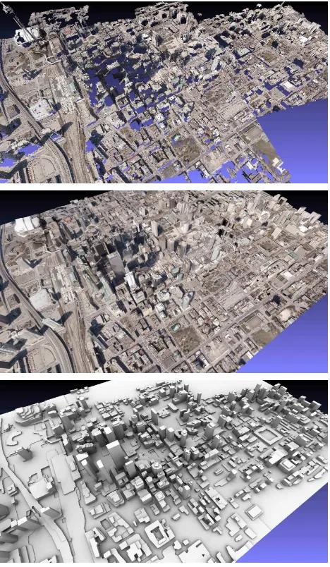
The proposed approach is evaluated on the Toronto dataset of the ISPRS Test Project on Urban Classification and 3D Building Re-construction (3D Scene Analysis, n.d.). This dataset includes roughly 1.45 km2 of the central area of Toronto, Canada. The aerial images have been acquired by Microsoft Vexcels UltraCam-D (UCUltraCam-D) camera. It contains typical structures of a modern North American city such as low- and high-story buildings but is rather challenging for MVS reconstructions as the overlap between im-ages is quite low. Figure 4 shows an example image.
Figure 5. Results of the proposed approach on the Toronto dataset. Top: Original input point cloud containing noise, outliers, and large missing regions; Middle: The obtained 3D city model with filled regions and removed outliers; Bottom: The
obtained untextured mesh as visualization of the pure geometry.
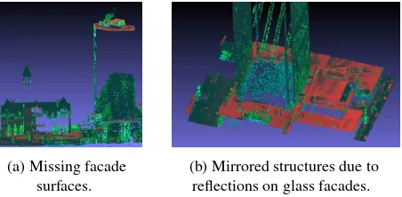
(a) Missing facade surfaces.
(b) Mirrored structures due to reflections on glass facades.
Figure 6. Missing and erroneous data in the provided reference data of the Toronto dataset1.
The Toronto dataset contains ALS data of the scene as reference data. The ALS data was acquired in February 2009 by Optechs ALTM-ORION M at an altitude of 650 m and has an approximate point density of 6.0 points/m2.
In principle, the availability of the ALS data allows a quantitative analysis. The corresponding performance metrics, however, have to be interpreted with a certain care for two major reasons.
1) The provided point cloud contains its own measurement er-rors as for example missing regions. In particular many of the facades, i.e. areas perpendicular to the ground plane are not avail-able (Figure 6a shows an example1). Another problem are ghost
structures, which are caused by reflecting parts of the scene such as glass elements on building facades. Figure 6b shows how a small building to the left of the skyscraper is placed within the skyscraper.
Furthermore, the images and the point cloud have been acquired at different dates. The time delay between both acquisitions caused that certain parts of the acquired data are different. One example are construction sites such as shown in Figure 7a. Although not being completely finished during point cloud acquisition (as in-dicated by the construction cranes on top), a building is clearly visible in the ALS scene. The images of the same part of the city, however, show merely an empty place. Another example is veg-etation, such as parks, which are clearly visible in the ALS data which was acquired during spring (see for example Figure 7b), but are not reconstructed by MVS. The images have been ac-quired earlier where trees had no leafs and the branches alone are too small to be considered by the reconstruction. Also smoke and steam as for example shown in Figure 7c are not reconstructed by MVS despite being visible in the ALS scan.
2) The overall goal of this work is not to obtain a highly accurate 3D reconstruction, but a meaningful abstraction of the scene to be used as a 3D city model. Abstractions, however, basically mean a reduction to the quintessence. The corresponding “loss” of preci-sion is therefore a necessary side effect and cannot be counted as an erroneous estimate. This renders any quantitative evaluation difficult, even if perfect ground truth data was available.
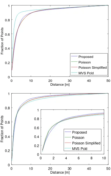
For reference we show the precision and completeness of the ob-tained mesh (with 30k faces), of a Poisson surface reconstruction (Kazhdan and Hoppe, 2013) (6.3M faces), of a simplification of the Poisson mesh (down to 100k faces), as well as of the original point cloud with respect to the ALS scan in Figure 8. To compute these measures, points are sampled randomly, but uniformly from the obtained meshes. While precision is the (average) minimal
1For better visualization, we colorize the ALS point cloud based on
intensity (red), number of reflections (green), and reflection index (blue).
(a) The construction of buildings not existent during image acquisition (left) has significantly proceeded during the ALS
scan (right).
(b) Trees apparent in the ALS scan (right) lost their leaves during fall when the images were acquired (left).
(c) Non-stationary signals such as steam (here from the ALS data) are generally not reconstructed by standard MVS methods.
Figure 7. Differences between reference ALS data and the image-based MVS reconstruction, mostly caused by large time
delay between data acquisitions1.
distance of a sampled point to a reference point, completeness states the (average) distance of a point in the reference data to the closest point in the sampled point cloud. In addition, for com-pleteness we also provide the slightly more common metric of the fraction of points whose distance is below a threshold (5m in our case). The values are listed in Table 1. In addition, complete cumulative histograms for precision and completeness are shown in Figure 8, which plot for all thresholds between zero and 50m the fraction of points whose distances are below that threshold.
As expected, the abstraction results in an increased error as can be seen in Table 1 and at the top of Figure 8. The average precision of the original point cloud lies at 3.2m, which decreased to 4.9m for both Poisson reconstructions and to 5.0m for the proposed approach (please note that smaller values mean higher precision).
0 10 20 30 40 50 0
0.2 0.4 0.6 0.8 1
Distance [m]
Fraction of Points
Proposed
Poisson
Poisson Simplified
MVS Pcld
0 10 20 30 40 50
0 0.2 0.4 0.6 0.8 1
Distance [m]
Fraction of Points
0 2 4 6 8 10
0 0.2 0.4 0.6 0.8 1
Proposed Poisson Poisson Simplified MVS Pcld
Figure 8. Quantitative results of the reconstruction. Top: Precision; Bottom: Completeness
Method Precision Completeness
Avg. (m) Avg. (m) %<5m
Proposed 5.00 3.43 82.8
Poisson 4.86 3.68 80.8
Poisson Simplified 4.89 3.76 80.3
MVS 3.22 4.12 79.6
Table 1. Average precision and completeness (ignoring distances>50m) on the Toronto dataset.
values mean higher completeness). The bottom of Figure 8 shows the cumulative histogram of completeness values. The first part of the histogram (shown enlarged) illustrates that less points in the reference point cloud have very small minimal distances (<3m) to points of the point cloud of the proposed approach. This is an effect of the abstraction that removes finer details in favour of a simplified geometry. For distances above 3 meters, the histogram illustrates that holes in the MVS point cloud are closed by all three surface reconstruction approaches, but more successfully by the proposed method.
Figure 9 shows where the errors (in terms of precision and com-pleteness) are originating. Both, the proposed approach as well as the input MVS point cloud suffer in terms of completeness from similar problems: New buildings, a small number of missed buildings, as well as vegetation seem to be the major sources of error. In terms of precision, the MVS point cloud performs quite well, except of course for regions where the scene changed. The proposed method, however, reconstructs the facades of the build-ings in addition to their roofs. Since those are not always part of the ALS data (or are severely undersampled), the facades are deemed very “imprecise” by the metric. A reference point cloud
0 m 10 m 20 m 30 m 40 m 50 m
Figure 9. Precision and completeness as color coded point clouds. Blue corresponds to a distance of zero, red to a distance of50m. From top to bottom: Precision of the proposed method, completeness of the proposed method, precision of the MVS
that contains all facades with adequate point density would be needed to derive a proper quantitative measure of completeness.
It should thus be noted again, that the quantitative results have to be taken with a grain of salt. First, the data related problems dis-cussed above (i.e. the differences between images and ALS scan) significantly contribute to the measurements above. Second, the goal of an abstraction is not an highly accurate reconstruction, but the creation of a realistic and visually pleasing, yet simplis-tic mesh, which maintains important geometric structures while keeping the geometry to a minimum. As Figure 5 illustrates, this goal has been achieved by the proposed method. An interactive view of the reconstruction is available at (Ley et al., 2017).
5. CONCLUSION AND FUTURE WORK
This paper applies prior work of interpreting the estimation of a dense depth map as a labelling problem to the task of 3D city modelling from aerial images. The depth map, which is turned into a height map in our top down use case, serves as an inter-mediate step for the construction of a simplified mesh which is as close as possible to the data while keeping the geometry to a minimum. In a last step, the obtained mesh is textured based on the input images.
In general, the approach performs well in the context of 3D city modelling. It results in visually pleasing abstractions of build-ings. Major geometric structures are maintained while clutter and noise are removed.
Despite its performance, the presented approach offers several possible extensions and improvements. The assumption of a (piece-wise) planar ground plane can be easily relaxed when a digital surface model of the scene is available.
Future work will focus on the usage of additional priors as for ex-ample symmetries, repetitions, and semantic information. Sym-metries, for example, can be encouraged by additional links of the MRF that connect pixels that should have the same label. Other constraints can easily be included in the energy of Equation 1. On the one hand, the data term can depend on semantic information for example to suppress vegetation from being part of the city model. On the other hand, the smoothness term can be altered to favor height jumps along certain lines such as borders of semantic objects.
Last but not least, the geometric model can itself be improved. At the moment only planes parallel to the ground plane are consid-ered, which led to the desired simplistic results. However, sloped planes, cones, and other typical roof shapes can easily be included in the framework.
ACKNOWLEDGEMENTS
This paper was supported by a grant (HE 2459/21-1) from the Deutsche Forschungsgemeinschaft (DFG). The authors would like to acknowledge the provision of the Downtown Toronto data set by Optech Inc., First Base Solutions Inc., GeoICT Lab at York University, and ISPRS WG III/4.
REFERENCES
3D Scene Analysis, n.d. http://www2.isprs.org/commissions/ comm3/wg4/tests.html.
Baillard, C., 2004. Production of dsm/dtm in urban areas: Role and influence of 3d vectors. In:ISPRS Congress, Vol. 35, p. 112.
Baillard, C. and Zisserman, A., 1999. Automatic line matching and 3d reconstruction of buildings from multiple views. In: IS-PRS Conference on Automatic Extraction of GIS Objects from Digital Imagery, Vol. 32, pp. 69–80.
Bignone, F., Henricsson, O., Fua, P. and Stricker, M., 1996. Au-tomatic extraction of generic house roofs from high resolution aerial imagery. In: European Conference on Computer Vision, pp. 85–96.
Boykov, Y., Veksler, O. and Zabih, R., 2001. Fast approximate energy minimization via graph cuts. IEEE Trans. on Pattern Analysis and Machine Intelligence23(11), pp. 1222–1239.
Chauve, A. L., Labatut, P. and Pons, J. P., 2010. Robust piecewise-planar 3d reconstruction and completion from large-scale unstructured point data. In:CVPR, pp. 1261–1268.
Chen, L., Teo, T., Shaoa, Y., Lai, Y. and Rau, J., 2004. Fusion of lidar data and optical imagery for building modeling. In: Inter-national Archives of Photogrammetry and Remote Sensing, Vol. 35, Part B4, pp. 732–737.
Cohen-Steiner, D., Alliez, P. and Desbrun, M., 2004. Variational shape approximation. In: ACM SIGGRAPH 2004 Papers, SIG-GRAPH ’04, pp. 905–914.
Cornelis, N., Leibe, B., Cornelis, K. and Gool, L., 2007. 3d urban scene modeling integrating recognition and reconstruction.
International Journal of Computer Vision78(2), pp. 121–141.
Fischer, A., Kolbe, T. and Lang, F., 1999. Integration of 2d and 3d reasoning for building reconstruction using a generic hierarchical model. In:Workshop on Semantic Modeling for the Acquisition of Topographic Information, pp. 101–119.
Furukawa, Y. and Ponce, J., 2010. Accurate, dense, and robust multi-view stereopsis.IEEE Trans. on Pattern Analysis and Ma-chine Intelligence32(8), pp. 1362–1376.
Furukawa, Y., Curless, B., Seitz, S. M. and Szeliski, R., 2009a. Manhattan-world stereo. In:CVPR, pp. 1422–1429.
Furukawa, Y., Curless, B., Seitz, S. M. and Szeliski, R., 2009b. Reconstructing building interiors from images. In:ICCV, pp. 80– 87.
Grompone von Gioi, R., Jakubowicz, J., Morel, J.-M. and Ran-dall, G., 2012. LSD: a Line Segment Detector.Image Processing On Line2, pp. 35–55.
Haala, N. and Anders, K., 1996. Fusion of 2d-gis and image data for 3d building reconstruction. In:International Archives of Photogrammetry and Remote Sensing, Vol. 31, pp. 289–290.
Haala, N. and Brenner, C., 1997. Generation of 3d city models from airborne laser scanning data. In:3rd EARSELWorkshop on Lidar Remote Sensing on Land and Sea, pp. 105–112.
Hui, L., Trinder, J. and Kubik, K., 2003. Automatic building extraction for 3d terrain reconstruction using interpretation tech-niques. In: ISPRS Workshop on High Resolution Mapping from Space, p. 9.
Ikehata, S., Yang, H. and Furukawa, Y., 2015. Structured indoor modeling. In:ICCV, pp. 1323–1331.
Kazhdan, M. and Hoppe, H., 2013. Screened poisson surface reconstruction.ACM Trans. Graph.32(3), pp. 29:1–29:13.
Ley, A. and Hellwich, O., 2016. Depth map based facade abstrac-tion from noisy multi-view stereo point clouds. In:GCPR.
Ley, A., H¨ansch, R. and Hellwich, O., 2017. Project Website. http://andreas-ley.com/projects/ AerialAbstraction/.
Maas, H. and Vosselman, G., 1999. Two algorithms for extracting building models from raw laser altimetry data.ISPRS Journal of Photogrammetry and Remote Sensing54, pp. 153–163.
Sinha, S. N., Steedly, D. and Szeliski, R., 2009. Piecewise planar stereo for image-based rendering. In:ICCV, pp. 1881–1888.
Sohn, G. and Dowman, I., 2007. Data fusion of high-resolution satellite imagery and lidar data for automatic building extraction.
ISPRS Journal of Photogrammetry and Remote Sensing62(1), pp. 43–63.
Suveg, I. and Vosselman, G., 2004. Reconstruction of 3d build-ing models from aerial images and maps.ISPRS Journal of Pho-togrammetry and Remote Sensing58(3-4), pp. 202–224.
Taillandier, F. and Deriche, R., 2004. Automatic buildings recon-struction from aerial images: a generic bayesian framework. In:
Proceedings of the XXth ISPRS Congress.
Vosselman, G., 1999. Building reconstruction using planar faces in very high density height data. In: ISPRS Conference on Au-tomatic Extraction of GIS Objects from Digital Imagery, Vol. 32, pp. 87–92.
Xiao, J., Fang, T., Zhao, P., Lhuillier, M. and Quan, L., 2009. Image-based street-side city modeling. In: ACM SIGGRAPH Asia 2009 Papers, SIGGRAPH Asia ’09, pp. 114:1–114:12.