ACCURACY ASSESSMENT OF RECENT GLOBAL OCEAN TIDE MODELS AROUND
ANTARCTICA
J. Leia, b, F. Lia, b, *, S. Zhanga, b, *, H. Kea, b, Q. Zhanga, b, W. Lia, b
a Chinese Antarctic Center of Surveying and Mapping, Wuhan University, Wuhan, China
b Collaborative Innovation Center for Territorial Sovereignty and Maritime Rights, Wuhan University, Wuhan, China jintao.lei @whu.edu.cn, [email protected], [email protected]
KEY WORDS: Ocean tide models, Antarctica, Altimeter, Accuracy
ABSTRACT:
Due to the coverage limitation of T/P-series altimeters, the lack of bathymetric data under large ice shelves, and the inaccurate definitions of coastlines and grounding lines, the accuracy of ocean tide models around Antarctica is poorer than those in deep oceans. Using tidal measurements from tide gauges, gravimetric data and GPS records, the accuracy of seven state-of-the-art global ocean tide models (DTU10、EOT11a、GOT4.8、FES2012、FES2014、HAMTIDE12、TPXO8) is assessed, as well as the most widely-used conventional model FES2004. Four regions (Antarctic Peninsula region, Amery ice shelf region, Filchner-Ronne ice shelf region and Ross ice shelf region) are separately reported. The standard deviations of eight main constituents between the selected models are large in polar regions, especially under the big ice shelves, suggesting that the uncertainty in these regions remain large. Comparisons with in situ tidal measurements show that the most accurate model is TPXO8, and all models show worst performance in Weddell sea and Filchner-Ronne ice shelf regions. The accuracy of tidal predictions around Antarctica is gradually improving.
* Corresponding author, Li Fei, Email [email protected]
* Corresponding author, Zhang Shengkai, Email [email protected]
1. INTRODUCTION
Caused by gravitational attraction between the Earth and other celestial bodies, ocean tide describes the rise and fall of sea water, and has periodic characteristics due to the cyclical influence of the Earth’s rotation. From coastal flooding to tidal dynamics, from the satellite altimetry to the satellite gravimetry, a deep understanding of ocean tide is needed (Chen 1980, Gu et al. 1999, Visser et al. 2010). Ocean tide models are usually used to provide corrections to GPS, altimeter or gravity data, which can later be adopted for further studies, such as ice mass balance or GIA. The prediction accuracy of ocean tide models is essential since the improvement of tidal corrections can effectively and correctly remove the tidal ‘noise’, so that the nontidal signals of interest can be studied more reliably (Bosch et al. 2009). Since the launch of T/P satellite, much progress in improving global tide models has been achieved (Fu et al. 1994). The satellite altimetry provides long-term, worldwide coverage tidal observations, which in turn promotes the development of tide research (The cm-level accuracy altimeter data needs an accurate knowledge of ocean tides). With the help of T/P satellite and the following Jason-1/2, ERS-1/2, ICESat satellites, as well as GPS measurements obtained on floating ice shelve and the GRACE gravimeter mission, dozens of global ocean tide models are developed by different teams or institutes. Thanks to the assimilation of T/P altimeter data and other tidal observation into models, the prediction accuracy of models in the deep oceans improve to 2-3 cm, but the accuracy in the Antarctic oceans does not mirror the same performance (Ray et al. 2011). The limitations in the Antarctica regions include but not limit to the 66° latitudinal coverage of T/P, the lack of bathymetric data under large ice shelves, the inaccurate definitions of coastlines and grounding lines, the poor knowledge of physical parameters such as bottom friction and viscous coefficient, the harsh environment impeding the obtainment of in situ tidal observations, and the big ice shelves
and seasonal ice sea where the uncertainty of altimetry data remains large (King and Penna, 2005a).
One of the most straightforward, convincing method of testing the modelling accuracy is to compare the model predictions with in situ tidal observations. For example, Baker and Bos (2002) used the gravimeters from the Global Geodynamics Project (GGP) to test 10 ocean tide models, and found that some of the ocean tide models showed big anomalous in some parts of the world. King et al. (2005b) found that their selected models shown disagreement by up to several decimeters per constituent in the large ice shelf regions in Antarctica, TPXO6.2 is the relative high-accuracy model at that time. Shum et al. (1997) and Stammer et al. (2014) made comprehensive and systematic assessments of global ocean tide models, they not only gave detailed evaluation of each ocean tide models, but also described future prospects for improvement. Although progress in tide modelling has been achieved due to the remarkable success of altimetry missions, the quantitative analysis is still needed, especially in the Antarctica where lack of validation data (Dubock et al. 2001, Zwally et al. 2002, Labroue et al. 2012). This paper focuses on the accuracy assessment of recent ocean tide models around Antarctica. Briefly introduction of selected models is given in section 2. Detailed assessments of precision between models and accuracy comparing to the in-situ data, as well as some discussion and analysis, are given in section 3 and 4, respectively. Summary and discussion are given in Section 4.
2. TIDE MODELS
from their prior models), while the last five are hydrodynamical models. The grid resolutions of these models vary from 1/30° to 1/2°. Different from Stammer et al. (2014), OSU12 model is not adopted in our study, since it has not yet covered the polar oceans and defaults to GOT4.8 at high latitudes (Fok 2012). FES2004 is taken as the representative model of classical and conventional models, to validate the accuracy improvement of state-of-the-art models in Antarctica. Each model includes eight major constituents, K1, K2, M2, N2, O1, P1, Q1, S2, and some also provide other constituents such as M4 and MS4. For consistency, Only the eight major constituents are assessed in our study.
2.1 DTU10
The DTU10 (Technical University of Denmark) model is based on an empirical correction to the FES2004 model using response method (Cheng and Andersen 2011). It identifies significant residual ocean tide signal in shallow waters and at high latitudes. The response method is used for along-track residual analysis of 18 year of data from the primary joint T/P, Jason-1/2 mission time series and 4 years of interleaved tracks of Topex/Jasion-1 interleaved mission. Outside the 66 parallel, combined Envisat, Geosat Follow-On, and ERS-2 data sets have been introduced to solve for the tides in the polar oceans. The eight major semidiurnal and diurnal tides are interpolated to a regular 1/8° by 1/8° grid using a depth-dependent interpolation method. The load tide is computed from FES2004.
2.2 EOT11a
EOT11a, which is used for reprocessing of GRACE gravity data, is a global model based on an empirical analysis of multi-mission satellite altimetry data, derived at Deutsches Geodätisches Forschungs Institut (Savcenko and Bosch 2012). Its tidal constituents are estimated based on a residual least squares harmonic analysis, and FES2004 is again used as the reference model to mitigate background noise caused by minor tidal constituents. The harmonic analysis is customized in order to improve the determination of shallow water tides. EOT11a
The GOT4.8 model belongs to the so-called Goddard/Grenoble Ocean Tide series (Ray 1999). It is based on the empirical tidal analysis of multisatellite altimeter data. The prior models were a combination of several global, regional and local tide models blended across their mutual boundaries. In the deep ocean between latitudes 66°, only T/P altimeter data was assimilated into the model; In shallow seas and polar oceans poleward of
66°, data from Geosat Follow-On, ERS-1/2, ICESat is used. Compared to its earlier GOT4.7 model, GOT4.8 corrects a problem with the dry-tropospheric correction that has been used in T/P Geophysical Data Records since the beginning of the mission. GOT4.8 has the coarsest spatial resolution of 1/2° by 1/2°, and the load tides are computed by an iterative method.2.4 FES series
Finite Element Solutions (FES) tidal atlases was produced by the French tidal group, led by C. Le Provost (Lyard et al. 2006). FES2004 model is produced from the CEFMO and CADOR
models. The spectral and finite element characteristics of the CEFMO model proved to be key factors for the success of the FES atlases, and the early introduction of loading and self-attraction terms in the tidal equation allowed to compute highly accurate hydrodynamic solutions for basin scale applications. FES2004 takes ice coverage into account in polar areas, and its gridded resolution is 1/8° by 1/8°. FES2004 is the conventional model recommended by IERS conventions.
FES2012 model takes advantage of longer altimeter time series, and is based on the solution of the tidal barotropic equations T-UGOm (Toulouse-Unstructured Grid Ocean model) using the ensemble, frequency domain SpEnOI (Spectral Ensemble Optimal Interpolation) data assimilation software (Carrere et al. 2012). With a new original high-resolution global bathymetry and a new global finite element grid, the ‘free’ solution of FES2012 is twice more accurate than FES2004. The spatial resolution is 1/16° by 1/16°. GOT4.8 tide loading is used to be fully compliant with the construction of the FES2012 atlas. FES2014 is the last version of the FES atlas improved from FES2012. FES2014 model takes advantage of longer altimeter time series and better altimeter standards, improved modelling and data assimilation techniques, a more accurate ocean bathymetry and a refined mesh in most of shallow water regions. Due to new global finite element grid, and the optimized assimilation of tidal gauges, the accuracy of FES2014 is improved compared to FES2012. The grid resolution of FES2014 is 1/16° by 1/16°, and the loading effects is computed using a preliminary version FES2014a.
2.5 HAMTIDE12
HAMTIDE12 model is based on the generalized inverse methods for tides, developed at the University of Hamburg (Taguchi et al. 2014). The principle of the HAMTIDE12 is the direct minimization of the model deficiency and the inaccuracy of the recordings in a least square sense, resulting to solve the over determined algebraic equations and so called normal equation, respectively. The equations are then solved by a memory saving iterative method for the given sparse matrix and the model is corrected simultaneously by inferring the physics from data. The dynamic residuals are then used for the detection of possible model errors such as bathymetry, parameterization of dissipation, loading and self-attraction (LSA) and so on. The spatial resolution of HAMTIDE12 is 1/8° by 1/8°.
2.6 TPXO8
TPXO8 model, developed at Oregon State University of United States, is the most recent tidal solutions produced using the representer-based variational scheme (Egbert and Erofeeva 2002). Primary data were harmonically analysed along-track tidal constants from T/P and Jason data, with load tide corrections based on the earlier assimilation solution of TPXO6.8. The TPXO8 atlas combines a basic global solution (TPXO8, obtained at 1/6° resolution) and over 30 high resolution local solutions using a weighted average of regional and global solutions over a narrow strip for a smooth transition to the global model in the open ocean. In particularly, 83 tide gauge data were assimilated around Antarctica. TPXO8 atlas is available in a multiresolution version, but the fixed 1/30° grid was used in all tests performed in our paper.
Table 1. Participating Global Ocean Tide Models
Model Type Country Resolution
/° Authors
EOT11a E Germany 1/8 Savcenko [2012]
E, empirical adjustment to an adopted model; H, assimilation into a barotropic hydrodynamic model
3. DIFFERENCES BETWEEN MODELS
Six models are selected to computed the standard deviation (One model from each kind, FES2014 was the representative of FES-atlas). First, all six selected models are resampled into the same 1/2° by 1/2° resolution. Then we used the following
equations to compute the Root Mean Square (
RMS
grid ) of each resampled grid of each model, and the correspondent RootSum Square (
RSS
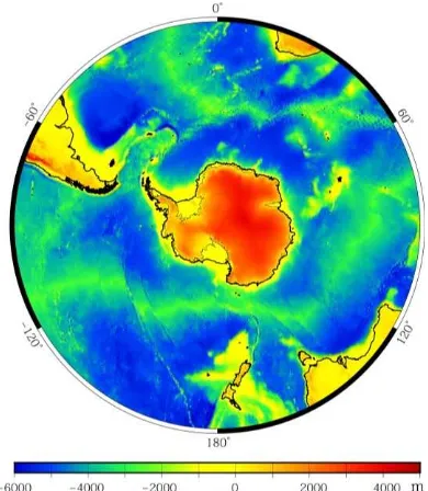
grid). 30°S, in order to show the real discrepancy between models, the down-weighted strategy of Stammer et al. (2014) was not adopted, instead, we use evenly weighted strategy. The results are separately listed in the table 2 for the Ice Shelf regions (including regions of permanent sea ice), the shallow seas (depth < 1000 m) and the deep ocean (depth > 1000 m), respectively. The depth comes from the 1/8° gridded bathymetry mask of Technical University of Denmark. Figure 1 is the bathygram.Table 2 shows that both RMS and RSS decrease in the order of Ice shelf regions, shallow seas and deep oceans. In the deep oceans, the RSS is 1.60 cm, which reaches the same level of the accuracy of T/P satellite. It means that present models agree well with each other over the deep oceans. The RSS of shallow
seas is 6.13 cm, twice bigger than of deep oceans. It means that due to the complex coastlines, bottom frictions and other factors, there are still some problems in the tide modelling in shallow seas. The RSS of models under the ice shelves are the largest, indicating that the uncertainties of models are relatively high. How to accurately model the ocean tide under the ice shelves are the biggest challenge nowadays. Comparing to the results of Stammer et al. (2014), all the RMS and RSS in our study are larger. This is due to the down weighted strategy Stammer et al. (2014) used. High latitudes over the coverage of T/P altimetry take larger proportion in our study, if the down weighted strategy was adopted, the RMS and RSS will be overly optimistic. For further discussion, the spatial patterns of the RMS and RSS of each constituents are displayed in Figure 2.
Figure 1. Bathygram of oceans southward of 30°S, the black lines are the coastlines, the grey lines in Antarctic are the
grounding lines (from Antarctic Digital Database http://www.add.scar.org/home/add7)
Table 2. RMS of differences between ocean tide models and their RSS /cm
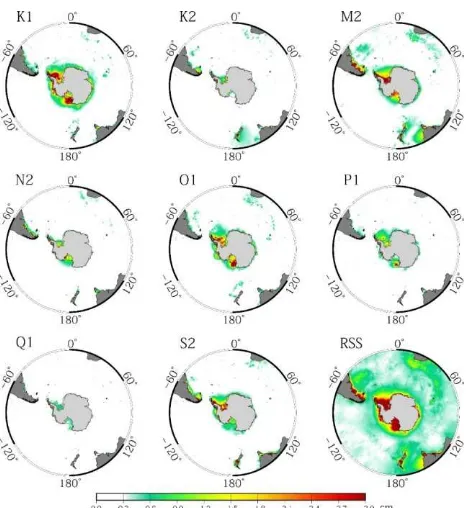
Depth K1 K2 M2 N2 O1 P1 Q1 S2 RSS Antarctica regions, Large discrepancy are found in the Weddell Seas, Ross Seas and under big ice shelves. Because of the coverage limitation of T/P altimetry, and obstacle of ice shelf and sea ice from the detection of other altimetry, the model predictions in the regions show the worst consistency. For semi-diurnal tides, the largest model discrepancies are located under big ice shelves, such as the Filchner-Ronne ice shelf and Ross ice shelf, and for the diurnal tides, the largest errors are in the open continental shelf areas of the western Ross and western Weddell Seas. Such an interesting finding is beyond the scope of this paper, and we remain it for future study.
also because of the different definition of coastlines and grounding lines, or the sparseness of spatial resolution.
Figure 2. The RMS and RSS for eight constituents between the six selected models. The spatial patterns of all constituents are
similar. For semi-diurnal tides, the largest discrepancies are located under big ice shelves, and for the diurnal tides, the
largest errors are in the open continental shelf areas.
Figure 3. RSS between the six selected models, in order of increasing depth. The RSS decreases from 10.38 cm under the ice shelves, to under 4 cm in the deep oceans. (IS is short for ice
shelf and those permanent sea ice regions)
4. TEST AGAINST TIDE GAUGE DATA
Comparison with in situ tidal observations is one of the most straightforward, convincing method, that can provide the ‘real’ external accuracy information about tide models. Due to the geographical and environmental constraints, the tide gauges around Antarctica are scarce, only a total 108 tidal measurements are available, including 44 bottom pressure recorders, 9 coastal tide gauges, 33 GPS records, 12 gravimeters, 2 tiltmeters and 8 visual tide staff records. All derived tidal constituents, as well as the information about record length, measure type can be downloaded from the Antarctic Tide Gauge Database (http: //www.esr.org/antarctic_tg_index.html). The
gravimeter and tiltmeter records, generally being based on shorter and older records and a greater number of uncertain corrections used in the reduction, are expected to be less reliable. Unfortunately, the gravimeter records make up a large fraction of the Ross ice shelf records. Therefore, we have to use these data. Fortunately, the tide gauges are generally quality controlled, and we chose as many records as we can.
Figure 4. Locations of all tidal measurements. The circle at 66°S is the southern limit of T/P altimetry, dots stand for those
records longer than 100 days, and triangles stand for those records shorter than 100 days.
After removing some unsuited measurements (distance too far away from Antarctica, or record time too short to be reliable). There are 86 tide gauge left for our tests. We used the bilinear interpolation to get the harmonic constants of eight models listed in table 1. The vector differences between in situ values and model predicted values are given by:
2
2 1/2mod mod mod mod
1 1
cos cos sin sin
2 el el 2 el el
Vector H G H G H G H G
(5)
Where
H
model andG
model are the amplitude and Greenwich phase lag of a constituent given by each model, respectively, andH
andG
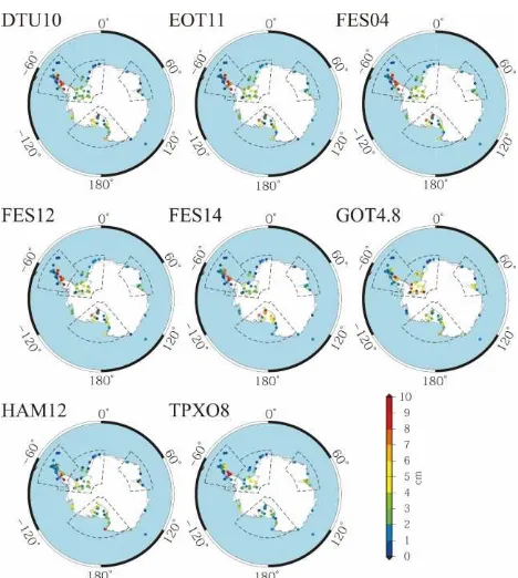
are the ‘ground truth’ amplitude and Greenwich phase lag observed by tide gauges, respectively.Figure 5 is he maps of vector differences between observed and bilinearly interpolated K1 signals. All eight models and their RSS show the similar spatial patterns, where the largest vectors are in the regions of Antarctic Peninsula and under the big ice shelves. According to the locations of in site data, we further divide the model performance analysis into four sub-regions, which are Antarctic Peninsula region, Amery ice shelf region, Filchner-Ronne ice shelf region and Ross ice shelf region. All results are listed in table 3-6. The RMS and RSS differences between the interpolated Antarctic Tidal signal and common tide gauges are computed by:
2 1/21
1
Nk tide k
RMS
VEC
N
(6)
1/ 28 2
1
1
8
k n
RSS
RMS
Where
VEC
tidek is the vector difference at a specific location, N is the total number of all tide gauges in one of four regions,RMS
k is the RMS of constituent k.Figure 5. Magnitudes of vector differences between observed and bilinearly interpolated K1 signals. All eight models and their RSS show the similar spatial patterns, where the largest vectors are in the regions of Antarctic Peninsula and under the
big ice shelves.
4.1 Antarctic Peninsula region
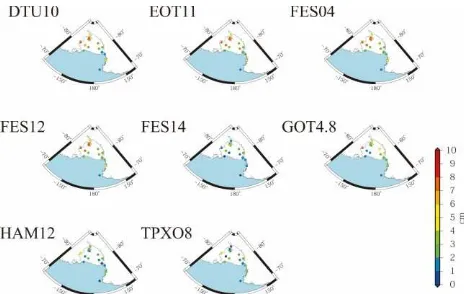
Figure 6. Magnitudes of vector differences between observed and bilinearly interpolated M2 signals for Antarctic Peninsula region. The spatial patterns of different models are similar, the
large vector differences are in the eastern part of Antarctic Peninsula, and their latitudes are always higher than others,
especially the Larsen C Ice shelf.
Figure 6 illustrates the maps of vector differences between observed and bilinearly interpolated M2 signals for Antarctic Peninsula region. The spatial patterns of different models are
similar, the large vector differences are in the eastern part of Antarctic Peninsula, and their latitudes are always higher than others, especially the Larsen C Ice shelf. From Figure 4 we know that some locations of tide gauges are within the coverage of T/P altimetry, and the correspondent prediction of models are more accurate, suggesting the importance of accurate altimeter data to the ocean tide modelling. The locations of several tide gauges with relatively large vector differences are not only out of the coverage of T/P altimetry, but also suffer from the permanent sea ice. The appearance of ice contaminates the accuracy of altimeter data, which seriously affects the modelling accuracy of ocean tide models.
Table 3. RMS between the interpolated tidal signal and common tide gauges for 4 major constituents, and the
correspondent RSS for 8 major constituents, in cm (Antarctic Peninsula region)
K1 M2 O1 S2 RSS
Num 30 30 30 27 - Mean Amp. 30.17 47.79 28.61 33.98 -
DTU10 5.57 3.77 4.63 4.40 9.96 (7.15) EOT11a 5.64 4.03 4.59 4.51 10.08 (7.24) FES2004 5.68 4.07 4.62 4.51 10.14 (7.41) FES2012 5.68 4.07 4.62 4.51 10.14 (7.39) FES2014 4.70 1.90 5.34 3.04 8.34 (4.89) GOT4.8 3.64 5.01 7.42 3.71 10.67 (5.95) HAMTIDE12 7.80 27.59 6.58 18.28 36.05 (6.67) TPXO8 6.36 5.26 3.39 3.96 10.40 (4.45) Num is the number of available data
Mean Amp. Is the mean amplitude of available data
Table 3 lists the RMS and RSS differences between the interpolated tidal signal and common tide gauges for Antarctic Peninsula region. We find that the HAMTIDE12 model has some difficulties in modelling the tides in this region, the RSS reaches over 30 cm, while the results of the other six models are very close to each other, with RSS at the level of 10 cm. FES2014 model, with its RSS of 8.34 cm, is the most accurate model in this region. Take a close look at the abnormal value of HAMTIDE12, we find that the problem occurs in the area of Larsen C ice shelf, where the vector differences of M2 can reach half a meter, even larger than the average amplitude (47.79 cm) of Antarctic Peninsula. We speculate that it may be the problem of assimilation method or the coastline geometry used in the HAMTIDE12 model. Therefore, care must be taken when using HAMTIDE12 model to do some research in the Antarctic Peninsula, especially near the Larsen C ice shelf. The last column in Table 3 also lists the RSS after removing the six tide gauges around Larsen C ice shelf (in brackets). After excluding the six abnormal gauges, RSS of all models decreases, and the most accurate model becomes the TPXO8, with RSS of 4.45 cm. The RSS of HAMTIDE12 comes to the same level of other models. Therefore, when using tide models in the Antarctic Peninsula, FES2014 model or TPXO8 model are recommended, and be careful to the performance of HAMTIDE12 model, especially near Larsen C ice shelf.
4.2
Amery ice shelf region
to the influence of ice shelf, the calculated vector differences on the ice shelf are at the level of 5 cm. Thanks to the locations of these gauges are in the middle of ice shelf, and not affected by the complex coastline or grounding line, there is no obvious abnormal value found in the region. There are three other tide gauges in the area far away from the Amery ice shelf, which are Syowa of Japan, Mawson and Davis of Australia. From Figure 7 it can be found that there is no obvious permanent sea ice near these tide gauges, so the modelling accuracy of all models are under 4 cm.
Figure 7. The same with Figure 6 but for Amery ice shelf Region. All calculated vector differences on the ice shelf are
under 5 cm.
Table 4. The same with Table 3, but for Amery ice shelf Region
K1 M2 O1 S2 RSS
Num 7 7 7 7 - Mean Amp. 27.72 19.30 28.24 19.44
DTU10 2.25 2.07 0.93 2.71 4.41 EOT11a 2.40 2.96 0.97 2.48 4.90 FES2004 2.41 2.97 0.99 2.48 4.97 FES2012 2.41 2.97 0.98 2.48 4.92 FES2014 2.44 3.34 1.70 3.33 6.59 GOT4.8 3.85 1.00 1.65 1.99 5.15 HAMTIDE12 2.09 1.20 1.05 1.92 3.54 TPXO8 3.50 2.05 2.33 3.48 6.06
Table 4 lists the RMS and RSS differences between the interpolated tidal signal and common tide gauges for Amery Ice Shelf region. Compared with table 3, the RMS and RSS values of Table 4 are small, suggesting the modelling accuracy of models in this region is higher than in Antarctic Peninsula. The minimum RSS is 3.54 cm, of HAMTIDE12 model, while the maximum RSS is 6.59 cm, of FES2014 model. HAMTIDE12 model is recommended to use for tidal study in this region.
4.3
Ross ice shelf region
Figure 8 shows a clear pattern that the vector differences increase with latitude increase. The largest vector differences can be found on the Ross Ice shelf, especially those regions close to the grounding lines, such as the southernmost tide gauges, where the grounding line pierces into the seas, accelerating the spatial variation of tides, resulting a large uncertainty in model predictions in the region.
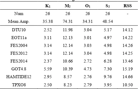
Table 5 lists the RMS and RSS values. Different from the Antarctica Peninsula and Amery ice shelf regions, the amplitudes of semi-diurnal constituents are small, the mean amplitudes of M2 and S2 constituents are less than 7 cm. But the RMS of these two constituents are large in this region compared to Table 4. Especially the M2 tide, its RMS reach up to about 5
cm, while its mean amplitude is only 6.59 cm. Therefore, the modelling accuracy in Ross seas is poorer than that in Amery regions. The RSS of TPXO8 model is 5.57 cm, significantly more accurate than other models. One of the reasons is that the TPXO8 model assimilates most of the tide gauges in this region. TPXO8 model is recommended in Ross Seas.
Figure 8. The same with Figure 6 but for Ross ice shelf region. It shows a clear pattern that the vector differences increase with
latitude increase.
Table 5. The same with Table 3, but for Ross ice shelf region
K1 M2 O1 S2 RSS
Num 17 17 17 17 - Mean Amp. 34.80 6.59 31.79 6.84
DTU10 4.93 4.74 5.26 2.48 10.39 EOT11a 4.99 4.94 5.37 2.24 10.51 FES2004 4.99 4.94 5.39 2.24 10.58 FES2012 4.99 4.94 5.39 2.24 10.52 FES2014 4.80 1.98 6.34 3.13 9.65 GOT4.8 3.27 3.56 9.32 2.79 11.36 HAMTIDE12 3.70 2.40 3.59 2.39 6.98 TPXO8 1.88 2.27 2.46 2.20 5.57
4.4
Filchner-Ronne ice shelf region
Figure 9. The same with Figure 6 but for Filchner-Ronne ice shelf region. This region has the worst performance in all four regions. Most large vector differences are located in the west of
the ice shelf, near the grounding line.
of M2 tide are larger than 10 cm, which is equivalent to the RSS values in other regions. Therefore, it makes the Filchner-Ronne ice shelf become the worst accurate region in all four regions. Most large vector differences are located in the west of the ice shelf, near the grounding line, where there are many ice streams, such as Evans Streams. The interaction between the ice streams and the ice shelf has an effect on the tidal measurement data, resulting in poor model prediction.
Table 6. The same with Table 3, but for Filchner-Ronne ice shelf region poor modelling accuracy in this area suggests that the effect of ice streams on the local tide modelling may be very powerful. The TPXO8 model has the best accuracy, with RSS of 10.50 cm, but the value is significantly larger than the its RSS in other regions. The worst model is GOT4.8, with RSS of 15.19 cm. The RSS of other models are more than 13 cm, indicating the modelling accuracy in this region need to be improved. TPXO8 model is recommended in this region.
4.5
Antarctic Seas
Table 7 lists the RMS and RSS differences between the interpolated tidal signal and common tide gauges for all Antarctic seas. From the above-mentioned problem, six tide gauges near Larsen C ice shelf are removed from our final analysis. All models have problems in producing the accurate tidal signal around Antarctica, especially in regions covered by the large ice shelves. All the models show vector differences of M2 larger than 10 cm on the Filchner-Ronne ice shelf, where the amplitude of M2 exceeds 1 m. The RMS differences for the full set of tide gauges range from 1 to 7 cm. Most models have large RSS on the Larsen C and Filchner-Ronne ice shelves in the Weddell sea. TPXO8 exhibits the lowest RMS for most constituents and clearly the lowest overall RSS, consistent with its assimilation of many of these in situ data records.
For DTU10, EOT11a and FES2004 models, their RMSs are all at the same level, as well as RSSs, which range from 10.23 cm to 10.38 cm. This is because both the DTU10 and EOT11a use the FES2004 as its a prior model. Even though DTU10 and EOT11a use longer data span and different techniques, the available observations and constraints data are limited, so they show no significant improvement compared to FES2004 around Antarctica. Therefore, in the process of modelling an empirical model, especially in the regions where lack of observations, the accuracy of a prior model is also very important, so care must be taken when selecting a priori model. For FES2004, FES2012
and FES2014 models, the RSSs are decrease from 10.38 cm to 9.57 cm, suggesting that the accuracy of the tide model is gradually increasing. When more and more data is available, we believe that the accuracy of tide models around Antarctic will gradually reach the same level as other continental shelf areas.
Table 7. The same with Table 3, but for all Antarctic Seas
K1 M2 O1 S2 RSS optimistic. HAMTIDE12 model exhibits a relatively high accuracy throughout the Antarctica, with overall RSS of 8.28 cm, which second to the TPXO8 model of 7.52 cm. But it is abnormal near Larsen C ice shelf, so it should be careful or avoided to use HAMTIDE12 model near the Larsen C ice shelf. TPXO8 model is recommended throughout the Antarctic seas.
5. SUMMARY
Using tidal measurements from tide gauges, gravimetric data and GPS records around the Antarctica, the accuracy of eight global ocean tide models is assessed. The standard deviations of eight major constituents from the selected models are large in polar regions, especially under the big ice shelves. Comparisons the model predictions with in situ tidal measurements show that the most accurate model is TPXO8, and all models show worst performance in Weddell sea and Filchner-Ronne ice shelf regions. And from the FES series models, we can find that the accuracy of tidal predictions around Antarctica is gradually improving.
ACKNOWLEDGEMENTS
This study is supported by the State Key Program of National Natural Science of China, No. 41531069, the Independent research project of Wuhan University, 2017, No. 2042017kf0209, the National Natural Science Foundation of China, No. 41176173, the Polar Environment Comprehensive Investigation and Assessment Programs of China, No. CHINARE2017.
REFERENCES
Baker T F, Bos M S. 2003. Validating Earth and ocean tide models using tidal gravity measurements. Geophysical Journal International, 152(2), pp. 468-485.
Bosch W, Savcenko R, Flechtner F, et al. 2009. Residual ocean tide signals from satellite altimetry, GRACE gravity fields, and hydrodynamic modelling. Geophysical Journal International, 178(3), pp. 1185-1192.
Carrère L, Lyard F, Cancet M, et al. 2012. FES 2012: a new tidal model taking advantage of nearly 20 years of altimetry measurements//Ocean Surface Topography Science Team 2012 meeting, Venice-Lido, Italy.
Chen Z., 1980. Tidology. Beijing: Science Press.
Cheng Y., Andersen O. B., 2011. Multimission empirical ocean tide modeling for shallow waters and polar seas. Journal of Geophysical Research: Oceans, 116(C11).
Dubock P. A., Spoto F., Simpson J., et al. 2001. The Envisat satellite and its integration. ESA bulletin, 106, pp. 26-45.
Egbert G. D., Erofeeva S. Y., 2002. Efficient inverse modeling of barotropic ocean tides. Journal of Atmospheric and Oceanic Technology, 19(2), pp. 183-204.
Fok H. S., 2012. Ocean tides modeling using satellite altimetry. The Ohio State University.
Fu L. L., Christensen E. J., Yamarone C. A., et al. 1994. TOPEX/POSEIDON mission overview. Journal of Geophysical Research: Oceans, 99(C12), pp. 24369-24381.
Gu Z., Jin W., Wang B., 1999. The comparison among ocean tide models and the ocean tide effect on the earth rotation.
Progress in Astronomy, 17(2): 126-135.
King M. A., Padman. L., 2005a. Accuracy assessment of ocean tide models around Antarctica. Geophysical Research Letters, 32(23).
King M. A., Penna N. T., Clarke P. J., et al. 2005b. Validation of ocean tide models around Antarctica using onshore GPS and gravity data. Journal of Geophysical Research: Solid Earth, 110(B8).
Labroue S., Boy F., Picot N., et al., 2012. First quality assessment of the Cryosat-2 altimetric system over ocean.
Advances in Space Research, 50(8), pp. 1030-1045.
Lyard F., Lefevre F., Letellier T., et al. 2006. Modelling the global ocean tides: modern insights from FES2004. Ocean Dynamics, 56(5-6), pp. 394-415.
Ray R. D., Egbert G. D., Erofeeva S. Y., 2011. Tide predictions in shelf and coastal waters: Status and prospects//Coastal altimetry. Springer Berlin Heidelberg, pp. 191-216.
Ray R. D., 1999. A global ocean tide model from TOPEX/ POSEIDON altimetry: GOT99. 2. NASA Tech. Memo. 209478, 58 pp., Goddard Space Flight Center, Greenbelt, MD.
Savcenko R., Bosch W., 2012. EOT11a—empirical ocean tide model from multi-mission satellite altimetry, DGFI Report No. 89, Deutsches Geodatisches Forschungsinstitut, Munchen.
Shum C. K., Woodworth P. L., Andersen O. B., et al. 1997. Accuracy assessment of recent ocean tide models. Journal of Geophysical Research: Oceans, 102(C11), pp. 25173-25194.
Stammer D., Ray R. D., Andersen O. B., et al. 2014. Accuracy assessment of global barotropic ocean tide models. Reviews of Geophysics, 52(3), pp. 243-282.
Taguchi E., Stammer D., Zahel W., 2014. Inferring deep ocean tidal energy dissipation from the global high-resolution data-assimilative HAMTIDE model. Journal of Geophysical Research: Oceans, 119(7), pp.4573-4592.
Visser P., Sneeuw N., Reubelt T., et al. 2010. Space-borne gravimetric satellite constellations and ocean tides: aliasing effects. Geophysical Journal International, 181(2), pp. 789-805.
Zwally H. J., Schutz B., Abdalati W., et al., 2002. ICESat's laser measurements of polar ice, atmosphere, ocean, and land.