Equivariant Counts of Points of the
Moduli Spaces of Pointed Hyperelliptic Curves
Jonas Bergstr¨om
Received: June 18, 2008 Revised: March 27, 2009
Communicated by Thomas Peternell
Abstract. We consider the moduli spaceHg,nofn-pointed smooth
hyperelliptic curves of genus g. In order to get cohomological in-formation we wish to make Sn-equivariant counts of the numbers of
points defined over finite fields of this moduli space. We find recur-rence relations in the genus that these numbers fulfill. Thus, if we can make Sn-equivariant counts of Hg,n for low genus, then we can
do this for every genus. Information about curves of genus 0 and 1 is then found to be sufficient to compute the answers forHg,n for all
g and for n ≤7. These results are applied to the moduli spaces of stable curves of genus 2 with up to 7 points, and this gives us the Sn-equivariant Galois (resp. Hodge) structure of their ℓ-adic (resp.
Betti) cohomology.
2000 Mathematics Subject Classification: 14H10, 11G20
Keywords and Phrases: Cohomology of moduli spaces of curves, curves over finite fields.
1. Introduction
By virtue of the Lefschetz trace formula, counting points defined over finite fields of a space gives a way of finding information on its cohomology. In this article we wish to count points of the moduli space Hg,n of n-pointed
smooth hyperelliptic curves of genusg. On this space we have an action of the symmetric group Sn by permuting the marked points of the curves. To take
this action into account we will makeSn-equivariant counts of the numbers of
points ofHg,n defined over finite fields.
For everynwe will find simple recurrence relations in the genus, for the equi-variant number of points of Hg,n defined over a finite field. Thus, if we can
characteristic is odd or even and the respective recurrence relations will in some cases be different.
When the number of marked points is at most 7 we use the fact that the base cases of the recurrence relations only involve the genus 0 case, which is easily computed, and previously known Sn-equivariant counts of points of
M1,n, to get equivariant counts for every genus. If we consider the odd and
even cases separately, then all these counts are polynomials when considered as functions of the number of elements of the finite field. For up to five points these polynomials do not depend upon the characteristic. But for six-pointed hyperelliptic curves there is a dependence, which appears for the first time for genus 3.
By the Lefschetz trace formula, the Sn-equivariant count of points ofHg,n is
equivalent to the trace of Frobenius on the ℓ-adicSn-equivariant Euler
char-acteristic of Hg,n. But this information can also be formulated as traces of
Frobenius on the Euler characteristic of some natural local systemsVλonHg.
By Theorem 3.2 in [1] we can use this connection to determine the Euler char-acteristic, evaluated in the Grothendieck group of absolute Galois modules, of all Vλ on Hg ⊗Q of weight at most 7. These result are in agreement with
the results on the ordinary Euler characteristic and the conjectures on the mo-tivic Euler characteristic ofVλonH3by Bini-van der Geer in [5], the ordinary Euler characteristic of Vλ on H2 by Getzler in [16], and the S2-equivariant cohomology ofHg,2 for allg≥2 by Tommasi in [20].
The moduli stack Mg,n of stable n-pointed curves of genus g is smooth and
proper, which implies purity of the cohomology. If theSn-equivariant count of
points of this space, when considered as a function of the number of elements of the finite field, gives a polynomial, then using the purity we can determine theSn-equivariant Galois (resp. Hodge) structure of its individualℓ-adic (resp.
Betti) cohomology groups (see Theorem 3.4 in [2] which is based on a result of van den Bogaart-Edixhoven in [6]). All curves of genus 2 are hyperelliptic and hence we can apply this theorem toM2,n for alln≤7. These results on genus
2 curves are all in agreement with the ones of Faber-van der Geer in [9] and [10]. Moreover, forn≤3 they were previously known by the work of Getzler in [14, Section 8].
Acknowledgements
The method I shall use to count points of the moduli space of pointed hyperel-liptic curves follows a suggestion by Nicholas M. Katz. I thank Bradley Brock for letting me read an early version of the article [7], and Institut Mittag-Leffler for support during the preparation of this article. I would also like to thank my thesis advisor Carel Faber.
Outline
⋆2 In this section we define Sn-equivariant counts of points ofHg,n over
a finite fieldk, and we formulate the counts in terms of numbers aλ|g,
which are connected to the H1’s of the hyperelliptic curves.
⋆3 The hyperelliptic curves of genusg, in odd characteristic, are realized as degree 2 covers of P1 given by square-free polynomials of degree 2g+ 2 or 2g+ 1. The numbersaλ|gare then expressed in terms of these
polynomials in equation (3.2). The expression foraλ|g is decomposed
into parts denotedug, which are indexed by pairs of tuples of numbers
(n;r). The special cases of genus 0 and 1 are discussed in Section 3.1. ⋆4 A recurrence relation is found for the numbers ug (Theorem 4.12).
The first step is to use the fact that any polynomial can be written uniquely as a monic square times a square-free one. This results in an equation which gives Ug in terms ofuh for hless than or equal to g,
where Ug denotes the expression corresponding to ug, but in terms of
all polynomials instead of only the square-free ones. The second step is to use that, ifgis large enough,Ug can be computed using a simple
interpolation argument.
⋆5 The recurrence relations for theug’s are put together to form a linear
recurrence relation for aλ|g, whose characteristic polynomial is given
in Theorem 5.2.
⋆6 It is shown how to computeu0 for any pair (n;r).
⋆7 Information on the cases of genus 0 and 1 is used to compute, for allg, ug for tuples (n;r) of degree at most 5, andaλ|g of weight at most 7.
⋆8 The hyperelliptic curves are realized, in even characteristic, as pairs (h, f) of polynomials fulfilling three conditions. The numbers ug and
Ug are then defined to correspond to the case of odd characteristic.
⋆9 In even characteristic, a recurrence relation is found for the numbersug
(Theorem 9.11). Lemmas 9.6 and 9.7 show that one can do something in even characteristic corresponding to uniquely writing a polynomial as a monic square times a square-free one in odd characteristic. This results in a relation between Ug and uh forhless than or equal to g.
Then, as in odd characteristic, a simple interpolation argument is used to computeUg forg large enough.
⋆10 The same amount of information as in Section 7 is obtained in the case of even characteristic. It is noted that aλ|g is independent of
the characteristic for weight at most 5 (Theorem 10.3). This does not continue to hold for weight 6 where there is dependency for genus at least 3 (see Example 10.6).
⋆11 The counts of points of the previous sections are used to get cohomo-logical information. This is, in particular, applied toM2,nforn≤7.
⋆12 In the first appendix, a more geometric interpretation is given of the information contained in all the numbersugof at most a certain degree
(see Lemma 12.8).
of the cohomology of sufficiently high weight, of some local systemsVλ
onHg. We will also see that these results are, in a sense,stable in g.
2. Equivariant counts
Letkbe a finite field withqelements and denote bykma degreemextension.
DefineHg,nto be the coarse moduli space ofHg,n⊗¯kand letFbe the geometric
Frobenius morphism.
The purpose of this article is to make Sn-equivariant counts of the number of
points defined over k of Hg,n. With this we mean a count, for each element
σ∈Sn, of the number of fixed points of F σ acting on Hg,n. Note that these
numbers only depend upon the cycle typec(σ) of the permutationσ.
Define Rσ to be the category of hyperelliptic curves of genus g that are
de-fined overktogether with marked points (p1, . . . , pn) defined over ¯ksuch that
(F σ)(pi) =pi for all i. Points of Hg,n are isomorphism classes of n-pointed
hyperelliptic curves of genus g defined over ¯k. For any pointed curve X that is a representative of a point in HF σ
g,n, the set of fixed points of F σ acting on
Hg,n, there is an isomorphism from X to the pointed curve (F σ)X. Using
this isomorphism we can descend to an element of Rσ (see [17, Lem. 10.7.5]).
Therefore, the number of ¯k-isomorphism classes of the categoryRσis equal to
|HF σ g,n|.
Fix an elementY = (C, p1, . . . , pn) inRσ. We then have the following equality
(see [12] or [17]):
X
[X]∈Rσ/∼=k X∼=k¯Y
1 |Autk(X)|
= 1.
This enables us to go from ¯k-isomorphism classes tok-isomorphism classes:
|Hg,nF σ|=
X
[Y]∈Rσ/∼=¯k
1 = X
[Y]∈Rσ/∼=k¯
X
[X]∈Rσ/∼=k X∼=¯kY
1 |Autk(X)|
= X
[X]∈Rσ/∼=k
1 |Autk(X)|
.
For any curveCoverk, defineC σto be the set ofn-tuples of distinct points (p1, . . . , pn) inC(¯k) that fulfill (F σ)(pi) =pi.
Notation 2.1. A partitionλ of an integer m consists of a sequence of non-negative integers λ1, . . . , λν such that |λ| := Pνi=1iλi = m. We will write
λ= [1λ1, . . . , νλν].
Say thatτ ∈Sn consists of onen-cycle. The elements ofC τ
are then given by the choice of p1 ∈ C(kn) such that p1 ∈/ C(ki) for every i < n. By an
inclusion-exclusion argument it is then straightforward to show that
|C τ|=X
d|n
µ(n/d)|C(kd)|,
where µis the M¨obius function. Say thatλis any partition and thatσ∈S|λ|
directly follows that
|elements and hence we obtain
(2.2) |Hg,nF σ|=
We will compute slightly different numbers than |HF σ
g,n|, but which contain
equivalent information. LetC be a curve defined overk. The Lefschetz trace formula tells us that for allm≥1,
If we consider equations (2.1) and (2.2) in view of equation (2.3) we find that
|HF σ
xi degreei. Then there is a unique monomial infσ of highest degree, namely
xλ1
1 · · ·xλνν. The numbers which we will pursue will be the following. Definition 2.2. Forg≥2 and any partition λdefine
(2.4) aλ|g :=
This expression will be said to haveweight |λ|. Let us also define a0|g:=
3. Representatives of hyperelliptic curves in odd characteristic
coordinate t = 1/x by y2 =t2g+2f(1/t). We will therefore let f(
∞), which corresponds tot= 0, be the coefficient off of degree 2g+ 2.
Definition 3.1. LetPg denote the set of square-free polynomials with
coeffi-cients inkand of degree 2g+ 1 or 2g+ 2, and letP′
g⊂Pg consist of the monic
polynomials. Write Cf for the curve corresponding to the elementf inPg.
By construction, there exists for eachk-isomorphism class of objects inHg(k)
an f in Pg such that Cf is a representative. Moreover, the k-isomorphisms
between curves corresponding to elements ofPgare given byk-isomorphisms of
their function fields. By the uniqueness of the linear systemg1
2on a hyperelliptic curve, these isomorphisms must respect the inclusion of the function field of P1. The k-isomorphisms are therefore precisely (see [16, p. 126]) the ones induced by elements of the groupG:= GLop2 (k)×k∗/D where
D:={( a 0 0 a
, ag+1) :a ∈k∗
} ⊂GLop2 (k)×k∗
and where an element
γ= [( a b c d
, e)]∈G induces the isomorphism
(x, y)7→
ax+b
cx+d, ey (cx+d)g+1
.
This defines a left group action of G on Pg, where γ ∈ G takes f ∈ Pg to
˜
f ∈Pg, with
(3.1) f˜(x) =(cx+d) 2g+2
e2 f
ax+b
cx+d
.
Notation 3.2. Let us putI:= 1/|G|= (q3
−q)−1(q
−1)−1.
Definition 3.3. Letχ2,m be the quadratic character on km. Recall that it is
the function that takesα∈kmto 1 if it is a square, to−1 if it is a nonsquare
and to 0 if it is 0. With a square or a nonsquare we will always mean a nonzero element.
Lemma 3.4. If Cf is the hyperelliptic curve corresponding tof ∈Pg then
am(Cf) =−
X
α∈P1(km)
χ2,m f(α).
Proof: The fiber of Cf → P1 over α ∈ A1(km) will consist of two points
defined overkm if f(α) is a square in km, no point if f(α) is a nonsquare in
km, and one point if f(α) = 0. By the above description off in terms of the
coordinatet= 1/x, the same holds forα=∞. The lemma now follows from
We will now rephrase equation (2.4) in terms of the elements ofPg. By what
was said above, the stabilizer of an element f in Pg under the action of Gis
equal to Autk(Cf) and hence
This can up to sign be rewritten as
(3.3) I X
will find recurrence relations ing.
Definition3.5. For any tuplen= (n1, . . . , nm)∈Nm≥1, let the setA(n) consist
Construction-Lemma 3.8. For each λ, there are positive integers c1, . . . , cs andm1, . . . , ms, and moreover pairs(n(i);r(i))∈ Nmi for each1≤i≤s, such
that for any finite field k,
aλ|g=
Proof: The lemma will be proved by writing the setS as a disjoint union of parts that only depend upon the partitionλ, and which therefore are indepen-dent of the chosen finite fieldk.
⋆ For each 1≤i≤ν, letTi,1, . . . , Ti,δi be an ordered partition of the set
{1, . . . , λi} into (possibly empty) subsets.
⋆ For each 1 ≤ i ≤ ν and each 1 ≤ j ≤ δi, let Qi,j,1, . . . , Qi,j,κi,j be
an unordered partition (where κi,j is arbitrary) of the set Ti,j into
non-empty subsets.
From such a choice of partitions we define a subset S′ = S(
{Ti,j},{Qi,j,k}) Definento be equal to the tuple
(
Definerto be equal to
(ρ1,1,1, ρ1,1,2, . . . , ρ1,1,κ1,1, ρ1,2,1, . . . , ρ1,δ1,κ1,δ1, ρ2,1,1, . . . , ρν,δν,κν,δν).
is clear in view of the following three simple properties of the quadratic char-acter.
S (for different choices of partitions{Ti,j}and{Qi,j,k}) are disjoint and cover
S.
The set of data {(ci,(n(i);r(i)))} resulting from the procedure given in the
proof of Construction-Lemma 3.8 is, after assuming the pairs (n(i);r(i)) to be distinct, unique up to simultaneous reordering of the elements of n(i) andr(i) for eachi, and it will be calledthe decomposition of aλ|g.
Definition 3.9. For a partitionλ, the pair
will appear in the decomposition ofaλ|g(corresponding to the partitionsTi,1= {1, . . . , λi} for 1 ≤i ≤ν, and Qi,1,k ={k} for 1 ≤i, k ≤ν) with coefficient
equal to 1, and it will be called thegeneral case. All other pairs (n;r) appearing in the decomposition ofaλ|g will be refered to asdegenerations of the general
case.
Definition 3.10. For any (n;r) ∈ Nm, the number |n| := Pmi=1ni will be
called thedegree of (n;r).
Lemma 3.11. The general case is the only case in the decomposition of aλ|g which has degree equal to the weight of aλ|g.
Proof: If (n;r) appears in the decomposition of aλ|g and is associated to
the partitions {Ti,j} and {Qi,j,k}, then |n|=Pνi=1
Pδi
j=1κi,jdi,j. Since λi =
Pδi
j=1κi,j and 1 ≤ di,j ≤i, the equality |λ| =|n| implies that κi,1 =λi and
κi,j= 0 ifj6= 1.
Lemma3.12.If(n;r)appears in the decomposition ofaλ|gthenPmi=1rini≤ |λ| and these two numbers have the same parity.
Proof: If (n;r) appears in the decomposition ofaλ|g and is associated to the
partitions{Ti,j}and{Qi,j,k}, thenPmi=1rini=Pνi=1Pδji=1Pκk=1i,j ρi,j,kdi,j.
Let us prove the lemma by induction on m, starting with the case that m =
Pν
i=1λi. In this case we must have |Qi,j,k| = 1 for all 1≤i≤ν, 1 ≤j ≤δi
and 1 ≤k≤κi,j, and hence ρi,j,k is only equal to two ifi/di,j is even. This
directly tells us that ρi,j,kdi,j ≤i, and that these two numbers have the same
parity. Since λi = Pδji=1κi,j, it follows that Pmi=1rini ≤ |λ| and that these
two numbers have the same parity.
Assume now thatm=kand that the lemma has been proved for all pairs (˜n; ˜r) with ˜m > k. Since m <Pνi=1λi we know that there exists numbersi0, j0, k0
such that |Qi0,j0,k0| ≥2. Let us fix an elementx∈Qi0,j0,k0 and define a new pair (n′;r′) associated to the partitions {T′
i,j}and{Q′i,j,k} by putting:
⋆ T′
i,j=Ti,j for all 1≤i≤ν and 1≤j≤δi,
⋆ Q′
i0,j0,k0 =Qi0,j0,k0\ {x}, ⋆ κ′
i0,j0 =κi0,j0+ 1 andQ
′
i0,j0,κ′i 0,j0
={x}, ⋆ Q′
i,j,k=Qi,j,k in all other cases.
The pair (n′,r′) thus appears in the decomposition of λ, and m′ = k+ 1.
Moreover, we directly find that Pmi=1rini ≤ Pm
′
i=1ri′n′i and that these two
numbers have the same parity. By the induction hypothesis the lemma is then
also true for (n;r).
Example 3.13. Let us decomposea[22]|g starting with the general case:
a[22]|g =I
X
f∈Pg
−X
α∈P1(k2)
χ2,2 f(α) 2
=I X
f∈Pg X
α,β∈P1(k2)
χ2,2 f(α)f(β)=
Example 3.14. The decomposition ofa[14,2]|g, starting with the general case: a[14,2]|g=−ug((2,1,1,1,1);(1,1,1,1,1))−6ug((2,1,1,1);(1,2,1,1))−3u((2g ,1,1);(1,2,2)) −4u((2g ,1,1);(1,1,1))−ug((2,1);(1,2))−ug((1,1,1,1,1);(2,1,1,1,1))−6ug((1,1,1,1);(2,2,1,1))
−4u((1g ,1,1,1),(1,1,1,1))−3ug((1,1,1);(2,2,2))−22u((1g ,1,1);(2,1,1))
−7u((1g ,1);(2,2))−8ug((1,1);(1,1))−u((1);(2))g .
3.1. The cases of genus0 and1. We would like to have an equality of the same kind as in equation (3.2), but for curves of genus 0 and 1. Every curve of genus 0 or 1 has a morphism toP1of degree 2 and in the same way as for larger genera, it then follows that everyk-isomorphism class of curves of genus 0 or 1 has a representative among the curves coming from polynomials in P0 andP1 respectively. But there is a difference, compared to the larger genera, in that for curves of genus 0 or 1 theg1
2is not unique. In fact, the groupGinduces (in the same way as for g ≥2) all k-isomorphisms between curves corresponding to elements ofP0 andP1that respect their given morphisms toP1 (i.e a fixed g1
2), but not allk-isomorphisms between curves of genus 0 or 1 are of this form. Let us, for allr≥0, define the categoryArconsisting of tuples (C, Q0, . . . , Qr)
where C is a curve of genus 1 defined overk and the Qi are, not necessarily
distinct, points onC defined over k. The morphisms of Ar are, as expected,
isomorphisms of the underlying curves that fix the marked points. Note that A0 is isomorphic to the categoryM1,1(k). We also define, for allr ≥0, the
categoryBrconsisting of tuples (C, L, Q1, . . . , Qr) of the same kind as above,
but whereLis ag1
2. A morphism ofBris an isomorphismφof the underlying
curves that fixes the marked points, and such that there is an isomorphismτ making the following diagram commute:
C −−−−→φ C′
L
y
yL′
P1 −−−−→τ P1.
ConsiderP1 as a category where the morphisms are given by the elements of G. To every element of P1 there corresponds, precisely as for g ≥2, a curve Cf together with a g21 given by the morphism to P1, thus an element of B0. Since every morphism in B0 between objects corresponding to elements ofP1 is induced by an element ofG, and since for everyk-isomorphism class of an element inB0 there is a representative inP1, the two categoriesP1andB0 are equivalent.
For allr≥1 there are equivalences of the categoriesAr andBrgiven by
(C, Q0, . . . , Qr)7→(C,|Q0+Q1|, Q1, . . . , Qr),
with inverse
We therefore have the equality
with q elements and for any curve C defined over k of genus g. For genus 1 this implies that|C(k)| ≥q+ 1−2√q >0, and thus every genus 1 curve has a point defined overk. There is therefore a number s such that 1≤ |C(k)| ≤s for all genus 1 curves C. As in the argument preceding equation (2.2) we can take a representative (C, Q0, . . . , Qr) for each element ofAr/∼=k and act with
Autk(C, Q0), respectively for each representative (C, L, Q1, . . . , Qr) ofB0/∼=k
act with Autk(C, L), and by considering the orbits and stabilizers we get s
Since this holds for all r≥1 we can, by a Vandermonde argument, conclude that we have an equality as above for each fixed j. We can therefore extend Definition 2.2 to genus 1 in the following way:
(3.4) aλ|1:=
which gives an agreement with equation (3.2).
All curves of genus 0 are isomorphic toP1 and ar(P1) = 0 for all r ≥1. In
this trivial case we just let equation (3.2) be the definition ofaλ|0.
4. Recurrence relations forug in odd characteristic
This section will be devoted to finding, for a fixed finite field k with an odd number of elements and for a fixed pair (n;r)∈ Nm, a recurrence relation for
ug. Notice that we will often suppress the pair (n;r) in our notation and for
instance writeug instead ofu(gn;r).
Fix a nonsquaretink and anα= (α1, . . . , αm)∈A(n). Multiplying with the
elementt gives a fixed point free action on the setPg and therefore
This computation and Lemmas 3.8 and 3.12 proves the following lemma.
Lemma 4.1. For any g≥ −1,(n;r)∈ Nm andα∈A(n), ifPmi=1rini is odd thenug,α= 0. Consequently,aλ|g is equal to0 if it has odd weight.
Thus, the only interesting cases are those for which Pmi=1rini is even.
Remark 4.2. The last statement of Lemma 4.1 can also be found as a conse-quence of the existence of the hyperelliptic involution.
We also see from equation (4.1) that
(4.2) ug,α=I(q−1)
Definition 4.3. LetQg denote the set of all polynomials (that is, not
neces-sarily square-free) with coefficients inkand of degree 2g+ 1 or 2g+ 2, and let Q′
g ⊂Qg consist of the monic polynomials. For a polynomial h∈Qg we let
h(∞) be the coefficient of the term of degree 2g+ 2 (which extends the earlier definition for elements in Pg). For any g ≥ −1, (n;r) ∈ Nm and α∈ A(n),
g large enough we will be able to computeUg. Together, this will give us our
recurrence relation forug.
With the same arguments as was used to prove equation (4.2) one shows that
(4.3) Ug,α=I(q−1)
of monic polynomials l of degreej such thatl(αi) is nonzero for alli. Let us
also put ˆbj = ˆbnj := Proof: The numbers bj can be computed by inclusion-exclusion, where the
choice of 1 ≤m1 < . . . < mi ≤m corresponds to demanding the polynomial
Notation 4.6. For anyα∈A′(n), letp
αi denote the minimal polynomial of
αi and putpα:=Qmi=1pαi.
i 6= j. The lemma now follows from the Chinese remainder theorem, which tells us that the morphism k[x]/pα → Qmi=1k[x]/pαi ∼=
Qm
i=1kni given by
f(x)7→(f(α1), . . . , f(αm)) is an isomorphism. Notation4.8. LetRj denote the set of polynomials of degreejand letRj′ be
the subset containing the monic polynomials. We will divide into two cases.
4.1. The case α ∈A′(n). Fix an element α
∈A′(n). Any nonzero
polyno-mial hcan be written uniquely in the form h=f l2 where f is a square-free polynomial and l is a monic polynomial. This statement translates directly into the equality this equality over allsbetween−1 andg gives
(4.5) Uˆg,α =
Summing this equality over allsbetween−1 andg gives (4.6) Uˆg,α=I(q−1)ˆb2g+2 forg≥ −1 if∀i:ri= 2.
In ˆUg,α we are summing over all polynomials h of degree less than or equal
to 2g+ 2, and every hcan uniquely be written on the form h1+pαh2, with
Using Lemma 4.7 we can reformulate this equality as
For anyj, half of the nonzero elements inkjare squares and half are nonsquares,
and thus ifri = 1 for somei, we can conclude from this equality that
(4.7) Uˆg,α= 0 forg≥(|n| −3)/2 if∃i:ri = 1.
4.2. The case α ∈ A(n)\A′(n). Fix an element α
∈ A(n)\A′(n). We
can assume that α1 = ∞, and then ˜α := (α2, . . . , αm) ∈ A′(˜n) where ˜n :=
(n2, . . . , nm).
Ifh∈Qg andf ∈Pj such thath=f l2for some monic polynomiall(which is
then unique), then h(∞) =f(∞), because the coefficient ofhof degree 2g+ 2 must equal the coefficient off of degree 2j+ 2. As in Section 4.1 we get (4.8)
Ug,α=I
X
j+k=g
X
l∈R′
j X
f∈Pk
f(∞)
m
Y
i=2
χ2,ni f(αi) ri
χ2,ni l(αi) 2ri
=
g+1
X
j=0 bn˜
jug−j,α.
IfPmi=1rini is even, equation (4.3) and the definition ofh(∞) shows that
(4.9) Ug,α=I(q−1)
X
h∈R′ 2g+2
m
Y
i=2
χ2,ni h(αi) ri
.
Ifri= 2 for alli, then equation (4.9) tells us that
(4.10) Ug,α =I(q−1)b˜n2g+2 forg≥ −1,∀i:ri= 2.
If 2g+ 2 ≥ |n| −1, an element h ∈ R′
2g+2 can be written uniquely as h = h1+p˜αh2, where deg(h1)≤ |n| −2, deg(h2)≥0 and h2 monic. In the same
way as in Section 4.1 we can (if Pmi=1rini is even) use this together with
equation (4.9) and Lemma 4.7 to conclude that
(4.11) Ug,α= 0 forg≥(|n| −3)/2,∃i:ri= 1,
which of course also holds ifPmi=1riniis odd by Lemma 4.1 and equation (4.8).
Remark 4.9. Fix anα∈ A(n). If there is an element β ∈ A1(k) such that β /∈ {α1, . . . , αn}, thenT(α) := (T(α1), . . . , T(αn)) is inA′(n), whereT is the
projective transformation ofP1
k defined byx7→βx/(x−β).
In the notation of equation (3.1), χ2,ni f(T(αi))
= χ2,ni f˜(αi)
(with e = 1). Since this induces a permutation of Pg, we find that ug,α =ug,T(α) and similarily thatUg,α =Ug,T(α). So, if q≥ |n|, then equations (4.5), (4.6) and
(4.7) will also hold forα∈A(n)\A′(n). By Lemma 4.10 in the next section,
we will see that this is true even ifq <|n|.
4.3. The two cases joined. In this section we will put the results of the two previous sections together using the following lemma.
Proof: Fix any tuplen= (n1, . . . , nm) and putn:=|n|. If we letti =qni in
then the right hand side is equal to the right hand side of equation (4.4), and hence
Proof: The theorem follows from combining equations (4.5), (4.6), (4.7) and equations (4.8), (4.10), (4.11), using Lemma 4.10. Note that with this theorem we can, for any (n;r)∈ Nm such thatri = 2 for
Forg≥(|n| −1)/2, Theorem 4.14 presents us with a linear recurrence relation forug which has coefficients that are independent of the finite fieldk.
Example4.15. If (n;r) = ((2,1,1,1); (1,2,1,1)) thenbn
5/(q−1) = (q2−1)(q− 1)2=q4−2q3+ 2q−1. Applying Lemma 4.13 and then Theorem 4.14 we get
ug−2ug−1+ 2ug−3−ug−4= 0 forg≥3.
Example 4.16. Let us compute ug, for all g ≥ −1, when (n;r) =
((1,1,1),(2,2,2)). We have that u−1 = J = 1 and since ri = 2 for all i,
Theorem 4.14 gives the equality u0 = 2u−1+J(q2−3q+ 1) = q2−3q+ 3. Applying Theorem 4.14 again we get
ug−2ug−1+ug−2=q2g−1(q−1)3 forg≥1. Solving this recurrence relation gives
u((1g ,1,1);(2,2,2))=
q2g+3(q
−1)−(2g+ 2)(q2
−1) + 3q+ 1
(q+ 1)2 forg≥ −1.
5. Linear recurrence relations for aλ|g
Remark5.1. From a sequencevn that fulfills a linear recurrence relation with
characteristic polynomialC we can, for any polynomialD, in the obvious way construct a linear recurrence relation forvnwith characteristic polynomialCD.
Thus, from two sequencesvn and wn that each fulfill linear recurence relation
with characteristic polynomialCandDrespectively, we can construct a linear recurence relation for the sequence vn +wn with characteristic polynomial
lcm(C, D).
Theorem 5.2. By applying Theorem 4.14 to each pair(n;r)appearing in the decomposition (given by Lemma 3.8) ofaλ|g, we get a linear recurrence relation for aλ|g. The characteristic polynomialC(X)of this linear recurrence relation equals
(5.1) 1
X−1
ν
Y
i=1
(Xi−1)λi.
Proof: Fix any pair (n;r) in the decomposition of aλ|g and put n = |n|.
Lemma 4.13 tells us that ˆbj −qˆbj−1 is equal to the coefficient of qn−1−j in bn/(q−1). If g ≥ n−1, then these numbers are also the coefficients
in the recurrence relation given by Theorem 4.14. By equation (4.12), the characteristic polynomial C(n;r) of this linear recurrence relation is equal to (Qmi=1(Xni−1))/(X−1).
We find that the linear recurrence relation in the general case (see Defini-tion 3.9) will have characteristic polynomial equal toC. Moreover, we find (by their construction in the proof of Lemma 3.8) that if (n;r) is a degenerate case thenC(n;r)|C. The theorem now follows from Remark 5.1.
Theorem 5.2 tells us that if we can compute aλ|g for g <|λ| −1 then we can
decomposition ofaλ|g we will do much better in Section 7, in the sense that we
will be able to use information from curves of only genus 0 and 1 to compute aλ|g for anyλsuch that|λ| ≤6.
Example5.3. Forλ= [14,2] the characteristic polynomial equals (X
−1)4(X+ 1), so ifVg is a particular solution to the linear recurrence relation fora[14,2]|g then
a[14,2]|g=Vg+A3g3+A2g2+A1g+A0+B0(−1)g, whereA0, A1, A2, A3and B0 do not depend upong.
6. Computing u0
In this section we will see that we can compute u0 for any choice of a pair (n;r)∈ Nm. This is due to the fact that if C is a curve of genus 0 then, for
where the base casen= 0 is trivial.
Let us put (˜n; ˜r) = ((n2, . . . , nm); (r2, . . . , rm)). For an ˜α = (α2, . . . , αm) ∈
Summing both sides of equation (6.2) over polynomialsf ∈P0 and using that an1(Cf) = 0 then gives
(6.3) u(0n;r)=−
X
i|n1
u(0n(i);r(i))−
X
ni|n1 niu(˜n;˜r
(i) ) 0 .
Since |n˜| < n and |n(i)| < n, the lemma follows by induction from
equa-tion (6.3).
Example 6.2. In the case (n;r) = ((6,6,3,1,1); (1,1,2,2,2)), the first step in the procedure in the proof of Lemma 6.1 equals
u(0n;r)=−u
((6,3,3,1,1);(1,2,2,2,2))
0 −u
((6,3,2,1,1);(1,2,1,2,2))
0 −u
((6,3,1,1,1);(1,2,2,2,2)) 0
−5u((60 ,3,1,1);(1,2,2,2))−6u((60 ,3,1,1);(2,2,2,2)).
Example6.3. In the case (n;r) = ((4,1,1,1); (1,2,1,1)), the procedure in the proof of Lemma 6.1 gives
u0(n;r)=u((20 ,1,1);(2,2,2))+u0((1,1,1);(2,2,2))+u((10 ,1);(2,2))−u((20 ,1);(2,2))−u((1);(2))0 7. Results for weight up to 7 in odd characteristic
We will in this section show that we, for any numbergand any finite fieldkof odd characteristic, can compute allaλ|g of weight at most 7. This is achieved
by decomposingaλ|gusing Lemma 3.8 and employing the recurrence relation of
Theorem 4.12 on the different parts. This involves finding the necessary base cases for the recurrence relations and that will be possible with the help of results on genus 0 curves obtained in Section 6, and on genus 1 curves obtained in the article [1].
We will writeaλ|g,oddandug,oddto stress that all results are in the case of odd
characteristic. See Section 10 for results in the case of even characteristic.
Example7.1. Theorem 4.12 is applicable even if the degree is 0 (if considered as a case whenri = 2 for alli) and with ˆbj=Pji=0qi. From Theorem 4.12 we find thata0|0,odd=Jq2=q/(q2−1) and again from Theorem 4.12 that
a0|g,odd=J(q2g+2−q2g) =q2g−1 forg≥1.
This result can also be found in [7, Proposition 7.1].
7.1. Degree at most 3. When the degree of the pair (n;r) is at most 3 we find using Theorem 4.12 that we do not need any base cases to computeugfor
everyg.
Example7.2. Let us consider (n;r) = ((2); (1)). We haveu−1=J= 1/(q+1) and applying Theorem 4.12 we getu0=−(q+ 1)u−1=−1. Theorem 4.14 tells us thatug=−ug−1 forg≥1 and thus
Example 7.3. The result fora[2]|g,odd is
a[2]|g,odd=−u((2);(1))g −u((1);(2))g = (−1)g−q2g forg≥0. Example 7.4. The result fora[12]|g,oddis
a[12]|g,odd=u((1g ,1);(1,1))+u((1);(2))g =−1 +q2g forg≥0.
Remark7.5. The result for (q2+ 1)a0|
g,odd−a[2]|g,oddcan be found in lecture
notes by Bradley Brock and Andrew Granville from 28 July 2003.
Example 7.6. Consider the case (n;r) = ((1,1,1); (2,1,1)). We haveu−1 = J = 1 and from Theorem 4.12 we getu0=−(q−2)u−1=−q+2. Theorem 4.14 gives the recurrence relationug= 2ug−1−ug−2 forg≥1 and hence
ug,odd((1,1,1);(2,1,1))=g(−q+ 1)−q+ 2.
7.2. Degree4 or5. From Theorem 4.12 we find that when the degree of the pair (n;r) is 4 or 5 we need the base case of genus 0. But the genus 0 case is always computable using Lemma 6.1 and then Theorem 4.12, and hence the same is true forug for allg.
Example 7.7. For (n;r) = ((2,1,1); (1,1,1)) we have u−1 = q and from Lemma 6.1 it follows that
u((20 ,1,1);(1,1,1))=−u
((2,1);(1,2))
0 =u
((1,1);(2,2))
0 +u
((1);(2)) 0 =q. Using Theorem 4.12 we get u1 =−(q−1)u0−(q2
−q−1)u−1 = −q3+ 2q. Solving the recurrence relationug=ug−1−ug−2−ug−3forg≥2, coming from Theorem 4.14, gives
u((2g,odd,1,1);(1,1,1))=1 4(q
3
−q)(−2g+ (−1)g−1) +q.
Example 7.8. The result fora[12,2]|g,odd is
a[12,2]|g,odd=−u((2g ,1,1);(1,1,1))−u((2g ,1);(1,2))−u((1g ,1,1);(2,1,1)) −u((1g ,1);(2,2))−2ug((1,1);(1,1))−u((1);(2))g =
=−q 2g+2
−1 q+ 1 −q
2g+1
2g(q 3+q
−2) +1 2
(
2q ifg≡0 mod 2 q3−q−2 ifg≡1 mod 2 7.3. Weight 6. We will not be able to computeug for all pairs (n;r) of
de-gree 6. But we will be able to compute ug for all pairs (n;r) that are general
cases in the decomposition of aλ|g forλ’s of weight 6. This will be sufficient
to compute all aλ|g of weight 6, because we saw in Lemma 3.11 that only the
general case will have degree 6 and therefore all degenerate cases are covered in Sections 7.1 and 7.2.
Let ug be the general case in the decomposition of aλ|g. When the degree is
equal to 6 we see from Theorem 4.12 that we need the base cases of genus 0 and 1 to computeug for all g. As we know, we can always compute u0 using
to 6 by the author. This was done by embedding every genus 1 curve with a given point as a plane cubic curve, see [1, Section 15]. Since we know all the degenerate cases in the decomposition ofaλ|1we can then compute the general caseu1.
Example 7.9. Let us deal with (n;r) = ((6); (1)) which is the generic case in the decomposition of a[6]|g,odd and for which we haveu−1 =J =q3+q−1. Using Lemma 6.1 we get
u((6);(1))0 =−u((3);(2))0 −u((2);(1))0 −u((1);(2))0 =−u((3);(2))0 =−q2. Using the results of [1, Section 15] we find that a[6]|1 =q−1. Decomposing a[6]|g gives a[6]|1 = −u((6);(1))1 −u
Example 7.10. The result fora[6]|g,odd is
a[6]|g,odd=−u((6);(1))g −u((3);(2))g −u((2);(1))g −u((1);(2))g =−q2g−
numberqof elements of the finite fieldkof odd characteristic. Ifλis of weight at most 7 it follows from our computations that this function is a polynomial in the variableq.
This will not continue to hold when considering for instancea[16]|3, that is, also including finite fields ofeven characteristic, see Example 10.6. But it will also not hold for instance fora[110]|1,odd, which for prime fields will be a polynomial function minus the Ramanujanτ-function, compare [15, Corollary 5.4].
8. Representatives of hyperelliptic curves in even characteristic
where handf are polynomials defined overk that fulfill the following condi-tions:
2g+ 1≤max 2 deg(h),deg(f)≤2g+ 2; (8.1)
gcd(h, f′2+f h′2) = 1; (8.2)
t∤gcd(h∞, f∞′2+f∞h′∞2).
(8.3)
The last condition comes from the nonsingularity of the point(s) in infinity, around which the curve can be described in the variable t = 1/x as y2 + h∞(t)y +f∞(t) = 0, where h∞ := tg+1h(1/t) and f∞ := t2g+2f(1/t). We
therefore define h(∞) and f(∞) to be equal to the degree g+ 1 and 2g+ 2 coefficient respectively. For a reference see for instance [19, p. 294].
Definition 8.1. Let Pg denote the set of pairs (h, f) of polynomials defined
overk, wherehis nonzero, that fulfill all three conditions (8.1), (8.2) and (8.3). WriteC(h,f)for the curve corresponding to the element (h, f) inPg.
To each k-isomorphism class of objects in Hg(k) there is a pair (h, f) in Pg
such that C(h,f) is a representative. All k-isomorphisms between the curves represented by elements of Pg are given by k-isomorphisms of their function
fields, and since the g1
2 of a hyperelliptic curve is unique the k-isomorphisms must respect the inclusion of the function field ofP1.
Identify the set of polynomialsl(x) defined overkand of degree at mostg+ 1 withkg+2, and define the group homomorphism
φg: GLop2 (k)×k∗→Aut(kg+2), φg(
a b
c d
, e) l(x):=
e−1(cx+d)g+1lax+b cx+d
.
Now define the groupGg:= kg+2⋊φg(GL
op
2 (k)×k∗)
/Dwhere
D:={(0, a 0 0 a
, ag+1) :a∈k∗} ⊂kg+2⋊φg (GL
op
2 (k)×k∗). Thek-isomorphisms between curves corresponding to elements of Pg are then
precisely the ones induced by elements ofGg by letting
γ= [(l(x), a b c d
, e)]∈Gg
induce the isomorphism
(x, y)7→ axcx++db, e y+l(x)
(cx+d)g+1
!
.
This defines a left group action of Gg onPg, where γ= [(l,Λ, e)]∈Gg takes
(h, f)∈Pg to (˜h,f˜)∈Pg, with
Definition 8.2. Let τm be the function that takes (a, b) ∈ k2m to 1 if the
equationy2+ay+bhas two roots defined overk
m, 0 if it has one root and−1
if it has none.
Lemma 8.3. If C(h,f) is the hyperelliptic curve corresponding to (h, f) ∈ Pg then
am(C(h,f)) =−
X
α∈P1(k
m)
τm h(α), f(α).
Proof: Follows in the same way as Lemma 3.4.
Notation 8.4. Let us putIg:= 1/|Gg|=q−(g+2)(q3−q)−1(q−1)−1.
In the same way as in the case of odd characteristic we get the equality
aλ|g=Ig
X
(h,f)∈Pg
ν
Y
i=1
− X
α∈P1(k
i)
τi h(α), f(α) λi
.
All results of Section 3.1 are independent of the characteristic and hence we extend the definition ofaλ|gto genus 0 and 1 in the same way as in that section. Definition 8.5. For anyg≥ −1, (n;r)∈ Nm andα∈A(n) define
u(n;r)
g,α :=Ig
X
(h,f)∈Pg
m
Y
i=1
τni h(αi), f(αi) ri
and
u(gn;r):=
X
α∈A(n) u(g,αn;r).
Construction-Lemma 8.6. For each λ we have (in even characteristic) the same decomposition of aλ|g as given by Construction-Lemma 3.8.
Proof: The following properties ofτmfor (h, f)∈Pg correspond precisely to
the ones for the quadratic character.
⋆ Say that α∈ P1(ks), then τ˜s h(α), f(α) =τs h(α), f(α)
2
if ˜s/sis even, and τ˜s h(α), f(α)=τs h(α), f(α)if ˜s/sis odd.
⋆ If for any α, β ∈ P1 we have Fs(α) = β for some s, then
τi h(α), f(α)
=τi h(α), f(β)
for alli. ⋆ Finally, for anyα∈P1 and anys, τ
,s h(α), f(α) r
=τs h(α), f(α)
2
ifris even andτs h(α), f(α) r
=τs h(α), f(α)ifris odd.
With this established we can use the same proof as for Construction-Lemma 3.8.
9. Recurrence relations for ug in even characteristic
Analogously to Section 4, this section will be devoted to finding for a fixed pair (n;r)∈ Nm, a recurrence relation forug. Fix ans∈kwhich does not lie in the
set{r2+r:r
∈k}, that is, such thatτ1(1, s) =−1. We define an involution on Pg sending (h, f) to (h, f+s h2). This involution is fixed point free and hence
ug,α=Ig
X
(h,f)∈Pg
m
Y
i=1
τni h(αi), f(αi) ri
=
=Ig
X
(h,f)∈Pg
m
Y
i=1
τni h(αi), f(αi) +s h
2(α
i)
ri
= (−1)Pmi=1riniu
g,α.
Thus, Lemma 4.1 also holds in the case of even characteristic.
Definition 9.1. Let Qg denote the set of pairs (h, f) of polynomials overk,
where his nonzero and h, f are of degree at mostg+ 1, 2g+ 2 respectively. Extending the definition forPg above to a pair (h, f)∈Qg, leth(∞) andf(∞)
be equal to the degreeg+ 1 and 2g+ 2 coefficient ofhandf respectively. For anyg≥ −1, (n;r)∈ Nmandα∈A(n) define
ˆ U(n;r)
g,α :=Ig
X
(h,f)∈Qg
m
Y
i=1
τni h(αi), f(αi) ri
and
ˆ Ug(n;r):=
X
α∈A(n) ˆ Ug,α(n;r).
Remark9.2. The connection between the setsQgandPgwhich we will present
below is due to Brock and Granville and can be found in an early version of [7]. There the connection is used to count the number of hyperelliptic curves in even characteristic, which is a0|g,even in our terminology.
Lemma9.3. Lethandf be polynomials overk. For any irreducible polynomial
m overk, the following two statements are equivalent:
⋆ m|gcd(h, f′2 +f h′2
);
⋆ there is a polynomial l overk, such thatm|handm2
|f+hl+l2.
Proof: Say that α∈kn is a root of an irreducible polynomialm and of the
polynomial gcd(h, f′2 +f h′2
). Letlbe equal tofqn/2
. Working modulo (x−α)2 we then get
f+hl+l2=f +hfqn/2+fqn
≡f(α) +f′(α)(x−α) +h′(α)f(α)qn/2(x−α) +f(α)qn ≡(x−α)(f′(α) +h′(α)f(α)qn/2)≡(x−α)(f′(α)2+h′(α)2f(α))1/2= 0, which tells us thatm2|f+hl+l2. For the other direction, assume that we have an irreducible polynomialmand a polynomiallsuch thatm|handm2
Differentiating the polynomial f +hl+l2 gives m2
|f′ +h′l+hl′, and thus
m|f′ +h′l. Taking squares we get m2
|f′2+h′2l2 and then it follows that m2
|f′2+h′2(f+hl) and hencem
|f′2+h′2f.
Let (h, f) be an element of Qg. In the first part of the proof of Lemma 9.3,
we may take forlany representative offqn/2
moduloh, because for theselwe havef +hl+l2 ≡f +hfqn/2
+fqn
modulo (x−α)2. In the second part it does not matter which degree l has. We conclude from this that Lemma 9.3 also holds if we assume thatl is of degree at mostg+ 1.
Chooseg≥ −1 and let (h, f)∈Qg. Lemma 9.3 gives the following alternative
formulation of the conditions (8.1), (8.2) and (8.3). For all polynomials l of degree at most g+ 1:
m|h, m2|f+hl+l2 =⇒ deg(m) = 0; (9.1)
deg(h) =g+ 1 or deg(f+hl+l2)≥2g+ 1. (9.2)
Here we used thatt|gcd(h∞, f∞′2+f∞h′∞2) if and only ift|h∞ and there exists
a polynomiall∞ such that deg(l∞)≤g+ 1 andt2|f∞+h∞l∞+l∞2 . In turn,
this happens if and only if deg(h)≤gand there exists a polynomiall of degree at mostg+ 1 such that deg(f+hl+l2)
≤2g, where we connectlandl∞using
the definitionsl:=xg+1l
∞(1/x) andl∞:=tg+1l(1/t).
This reformulation leads us to making the following definition.
Definition9.4. Let∼gbe the relation onQggiven by (h, f)∼g(h, f+hl+l2)
if l is a polynomial of degree at most g+ 1. This is an equivalence relation and since (h, f) = (h, f+hl+l2) if and only if l= 0 or l=h, the number of elements of each equivalence class [(h, f)]g isqg+2/2. If (h, f)∈Pg⊂Qg then
[(h, f)]g⊂Pg and we get an induced equivalence relation onPg which we also
denote∼g.
We will now construct all∼g equivalence classes of elements ofQg in terms of
the∼i equivalence classes of the elements inPi, whereiis between−1 andg.
This is the counterpart of factoring a polynomial into a square-free part and a squared part in the case of odd characteristic.
Definition 9.5. For z := [(h, f)]i ∈ Pi/ ∼i let Vz be the set of all
equiva-lence classes [(mh, m2f)]
ginQg for all monic polynomialsmof degree at most
g−i. This is well defined since if (h1, f1) ∼i (h2, f2) then (mh1, m2f1) ∼g
(mh2, m2f2).
Lemma 9.6. The setsVz for allz∈Pi/∼i where −1≤i≤g are disjoint. Proof: Say that for some z1 and z2 the intersection Vz1 ∩Vz2 is nonempty. That is, there exist (h1, f1)∈ Pi1, (h2, f2)∈ Pi2 and monic polynomials m1, m2 such that m1h1 = m2h2 and m2
factor of m1 is a factor of m2. The situation is symmetric and therefore the converse also holds.
So far we have not ruled out the possibility that a factor inm1 appears with higher multiplicity than in m2, or vice versa. Let m be the product of all irreducible factors of m1 and put ˜m1 :=m1/m, ˜m2 :=m2/m and ˜l := l/m. We are then in the same situation as above, that is ˜m1h1= ˜m2h2and ˜m2
1f1= ˜
m2
2f2+ ˜m2h2˜l+ ˜l2. Thus, if ris an irreducible polynomial such thatr|m1˜ but r ∤ m2˜ we can argue as above to conclude that r is constant. By a repeated application of this line of reasoning we can conclude thatm1 andm2 must be equal.
It now follows thath1=h2 and thatm2|l, thus (h1, f1)∼i1 (h2, f2). This tells us thatVz1∩Vz2 is only nonempty whenz1=z2.
Lemma 9.7. The setsVz for allz∈Pi/∼i where −1≤i≤g coverQg/∼g. Proof: Pick any element (h1, f1)∈Qgand putg1:=g. We define a procedure,
where at theith step we ask if there are any polynomialsmi and li such that
deg(mi) > 0, deg(li) ≤ gi+ 1, mi|hi and m2i|fi+hili +l2i. If so, take any
such polynomials mi,li and definehi+1:=hi/mi,fi+1:= (fi+hili+li2)/m2i
andgi+1:=gi−deg(mi). This procedure will certainly stop. Assume that the
procedure has been carried out in some way and that it has stopped at thejth step, leaving us with some pair of polynomials (hj, fj).
Next, we take (hj, fj+1) to be any element of the set [(hj, fj)]gj for which
deg(fj+1) is minimal. Say that fj+1 = fj +hjlj +l2j where deg(lj) ≤
gj + 1 and let us define gj+1 to be the number such that 2gj+1 + 1 ≤ max 2 deg(hj),deg(fj+1) ≤ 2gj+1+ 2. The claim is now that (hj, fj+1) ∈
Pgj+1. By definition, condition (8.1) holds for (hj, fj+1). If there were polyno-mialsmj+1andlj+1such thatmj+1|hj andm2j+1|fj+1+hjlj+1+l2j+1then the pair of polynomialsmj+1 andlj+lj+1would contradict that the process above stopped at thejth step. Hence condition (9.1) is fulfilled for (hj, fj+1).
Condi-tion (9.2) is fulfilled if 2 deg(hj)≥deg(fj+1) because then deg(hj) =gj+1+ 1. On the other hand, if 2 deg(hj) < deg(fj+1) and there were a polynomial lj+1 such that deg(lj+1) ≤ gj+1+ 1 and deg(fj+1+hjlj+1+lj2+1) ≤ 2gj+1 then this would contradict the minimality of deg(fj+1). We conclude that
(hj, fj+1)∈Pgj+1.
Finally we see that if we put ˆmr:=Qri=1−1miandl:=Pji=1mˆili, then deg(l)≤
g+ 1, h1 = ˆmjhj and f1 = ˆmj2fj+1+h1l+l2. This shows thatVz contains
[(h1, f1)]g wherez:= [(hj, fj+1)]gj+1∈Pgj+1/∼gj+1. Using the lemmas above we will be able to write ˆUgin terms ofuiforibetween
−1 and g. After this we will determine ˆUg for large enough values of g. We
divide into two cases.
Notation 9.8. Let Sj denote all polynomials of degree at most j, and let
S′
9.1. The case α ∈ A′(n). Fix an element α
∈ A′(n). It follows from
Lemma 9.6 and Lemma 9.7 that
(9.3) ˆUg,α=
Summing equations (9.5) and (9.6) over allh0∈Sg+1and using thatq2g+3Ig=
i and any monic polynomial m of degree g−i,
τs((mh)(∞),(m2f)(∞)) =τs(h(∞), f(∞));
τs((mh)(∞),(f +lh+l2)(∞)) =τs(h(∞), f(∞)).
Proof: Clear.
For any (h, f)∈Qgit holds that if deg(h)< g+ 1 thenτs(h(∞), f(∞)) = 0 for
alls. Define thereforeP′
g andQ′g to be the subsets ofPg andQg respectively,
that consist of pairs (h, f) such that deg(h) =g+1. We get an induced relation ∼ionPi′andQi′and we letVz′′be the set of all equivalence classes [(mh, m2f)]g
together with Lemma 9.10 and the arguments showing equation (9.4) we find that
then we find in the same way as for equation (9.6) that
9.3. The two cases joined. Recall thatJ = (q−1)I|A(n)|.
Theorem 9.11. For any pair(n;r)∈ Nm, g+1
X
j=0
ˆbjug−j=
(
J qg+1ˆb
g+1 if ∀i:ri = 2,g≥ −1;
0 if ∃i:ri = 1,g≥|n|−2 3.
Proof: The theorem follows from combining equations (9.4), (9.7), (9.8) and
(9.10), using Lemma 4.10.
Theorem 9.12. For any pair(n;r)∈ Nm,
min(|n|−1,g+1)
X
j=0
(ˆbj−qˆbj−1)ug−j=
(
J qg+1(ˆb
g+1−ˆbg) if ∀i:ri = 2,g≥0;
0 if ∃i:ri = 1,g≥|n|−2 1. Proof: In the notation of the proof of Theorem 4.14, the theorem follows from applying Theorem 9.11 to the expressionF(g)−qF(g−1).
Theorem 9.13. By applying Theorem 9.12 to each pair (n;r) appearing in the decomposition (given by Lemma 8.6) ofaλ|g,evenwe get a linear recurrence relation for aλ|g,even. The characteristic polynomial of this linear recurrence relation equals (5.1).
Proof: We know that the decomposition ofaλ|g is independent of
character-istic, and since the left hand side of the equation in Theorem 9.12 is the same as the left hand side of the equation of Theorem 4.14 this theorem follows in
the same way as Theorem 5.2.
10. Results for weight up to 7 in even characteristic
In this section we compute, for any numbergand any finite fieldkof even char-acteristic, allaλ|g,evenof weight at most 7. First we will exploit the similarities
of Theorems 4.12 and 9.11.
Lemma 10.1. Ifg≥n−2 thenb2ˆ g+2=qg+1ˆbg+1.
Proof: Fix a pair (n;r)∈ Nm. Lemma 4.13 tells us that ˆbj=qbˆj−1+d|n|−1−j,
so ifj≥ |n|then ˆbj=qˆbj−1 and thus ˆbj =qj+1−|n|ˆb|n|−1.
Remark 10.2. If ri = 1 for some i and g ≥ (|n| −3)/2, then the recursive
relations of Theorems 9.11 and 4.12 are equal. On the other hand, if ri = 2
for alliwe see from Lemma 10.1 that the recursive relations of Theorems 9.11 and 4.12 are equal ifg≥ |n| −2.
Proof: Consider anyaλ|gwith|λ| ≤5. By Lemma 3.12 it suffices to show that
ugis independent of characteristic when (n;r)∈ Nmis such thatPmi=1niri≤5.
Clearly u−1 =J is always independent of characteristic. Clearly, Lemma 6.1 also holds in even characteristic. We can therefore assume that ri = 2 for all
i in the case of genus 0. But if ri = 2 for all i then |n| ≤ 2 and hence, by
Remark 10.2,u0 will be independent of characteristic.
This takes care of the base cases of the recurrence relations forug wheng≥1,
given by Theorems 4.12 and 9.11. Again by Remark 10.2 we see that (both in the case when ri = 2 for all i, and when ri = 1 for some i) when g ≥ 1
these recurrence relations are the same. We can therefore conclude that ug is
independent of characteristic for allg.
We will now computeaλ|g,evenfor weight 6 in the same way as in Section 7.3.
To computeugof degree at most 5 using Theorem 9.11 we need to find the base
caseu0. But when the genus is 0 we can use Lemma 6.1 (which also holds in even characteristic) to reduce to the case that ri = 2 for alli, which is always
computable using Theorem 9.11.
What is left is the general case of the decomposition ofaλ|g,even. We then need
the base cases of genus 0 and 1. Again, the genus 0 part is no problem. The computation of aλ|1 in [1] is independent of characteristic. We can therefore compute the genus 1 part (compare Section 7.3).
Remark10.4. As in the case of odd characteristic, for allgand allλsuch that |λ| ≤7,aλ|g,even is a polynomial when considered as a function in the number
q(compare Remark 7.11) of elements of the finite fieldkof even characteristic. In Theorem 10.3 we saw that the polynomial functions aλ|g,odd and aλ|g,even
are equal (for a fixed g), if |λ| ≤ 5. But for weight 6 there are λ such that the two polynomials are different, this occurs for the first time for genus 3, see Example 10.6.
Example10.5. Let us computeug,evenwhen (n;r) = ((1,1); (2,2,2)). We see
thatu−1= 1 and Theorem 9.11 givesu0=q2−3q+ 2. This result is different from the 1 in the case of odd characteristic, see Example 4.16. Continued use of Theorem 9.11 gives u1 =q4
−3q3+ 5q2
−6q+ 3 and then Theorem 9.12 gives
ug= 2ug−1−ug−2+q2g−1(q−1)3 forg≥2. Solving this leaves us with
u((1g,even,1,1);(2,2,2))=
(q−1)(q2g+3+g(q2
−1)−3q−2)
(q+ 1)2 .
Example 10.6. The result fora[16]|g,even is
a[16]|g,even=a[16]|g,odd− 5
8g(g−1)(g−2) (g−3)(q−1)−4
Example 10.7. The result fora[12,4]|g,evenis
a[12,4]|g,even=a[12,4]|g,odd−1 4
g(q−1) ifg≡0 mod 4; (g−1)(q−1) ifg≡1 mod 4; (g−2)(q−1) ifg≡2 mod 4; (g−3)(q−1)−4 ifg≡3 mod 4.
11. Cohomological results
11.1. Cohomological results for Hg,n. Define the local system V :=
R1π
∗(Qℓ) where π : Mg,1 → Mg is the universal curve. For every
par-tition (note that in this section we use a different notation for parpar-titions) λ = (λ1 ≥ . . . ≥ λg ≥ 0) there is an irreducible representation of GSp(2g)
with highest weight (λ1−λ2)γ1+. . .+λgγg− |λ|η, where theγi are suitable
fundamental roots andη is the multiplier representation, and we defineVλ to
be the corresponding local system. Let us also denote by Vλ its restriction to
Hg. In Lemma 13.5 below we will see that making anSn˜-equivariant count of points of Hg,n˜ over a finite field k, for all ˜n ≤n, is equivalent to computing the trace of Frobenius on the compactly supportedℓ-adic Euler characteristic ec(Hg⊗k,¯ Vλ), for everyλwith |λ| ≤ n(whereℓ∤|k|). For more details, see
[14] and [15].
Thus, we can use the results of Section 7 together with Theorem 3.2 in [1] to compute the ℓ-adic Euler characteristic ec(Hg⊗Q,Vλ) in K0(GalQ), the
Grothendieck group of Gal( ¯Q/Q)-representations, for every λ with |λ| ≤ 7. Specifically, Theorem 3.2 in [1] tells us that if there is a polynomial P such that Tr(F,ec(Hg ⊗k,¯ Vλ)) = P(q) for all finite fields k, possibly with the
exception of a finite number of characteristics, then ec(Hg⊗Q,Vλ) = P(q),
where qis the class of Qℓ(−1) inK0(GalQ). By excluding even characteristic,
Section 7 (see Remark 7.11) and Lemma 13.5 shows that there is indeed such a polynomial for all gand all|λ| ≤7.
Example 11.1. Forg= 8 and λ= (5,1) we have
ec(Hg⊗Q,Vλ) = 5q5−28q4+ 4q3+ 96q2−34q−88.
11.2. Cohomological results for M2,n and M2,n. Using the
stratifica-tion ofMg,nwe can make anSn-equivariant count of its number of points using
theSn-equivariant counts of the points ofM˜g,n˜for all ˜g≤gand ˜n≤n+2(g−g)˜ (see [13, Thm 8.13] and also [2]). Since all curves of genus 2 are hyperelliptic, M2,n is equal to H2,n. Above, we have made Sn-equivariant counts of H2,n
forn≤7 and they were all found to be polynomial inq. TheseSn-equivariant
counts can now be complemented with ones ofM1,nforn≤9 (see [1, Section
15]) and of M0,n for n≤11 (see [18, Prop 2.7]), which are also found to be
polynomial in q. We can then apply Theorem 3.4 in [2] to conclude, for all n ≤ 7, the Sn-equivariant GalQ (resp. Hodge) structure of the ℓ-adic (resp.
In the theorems below we give the Sn-equivariant Hodge Euler characteristic
(which by purity is sufficient to conclude the Hodge structure) in terms of the Schur polynomials and L, the class of the Tate Hodge structure of weight 2 in K0(HSQ), the Grothendieck group of rational Hodge structures. That is,
the action of Sn on M2,n induces an action on its cohomology, and hence
Hi(
M2,n⊗C,Q) may be written as a direct sum ofHλi(M2,n⊗C,Q), which
correspond to the irreducible representations ofSn indexed byλ⊢nand with
charactersχλ. In terms of this, the coefficient of the Schur polynomial sλ is
equal to 1/χλ(id)·Pi(−1)i[Hλi(M2,n⊗C,Q)]. The results for n ≤ 3 were
previously known by the work of Getzler in [14, Section 8].
Theorem11.2. TheSn-equivariant Hodge Euler characteristic ofM2,4is equal
to
(L7+ 8L6+ 33L5+ 67L4+ 67L3+ 33L2+ 8L+1)s4 +(4L6+ 26L5+ 60L4+ 60L3+ 26L2+ 4L)s31 +(2L6+ 12L5+ 28L4+ 28L3+ 12L2+ 2L)s
22
+(3L5+ 10L4+ 10L3+ 3L2)s 212
Theorem11.3. TheSn-equivariant Hodge Euler characteristic ofM2,5is equal
to
(L8+ 9L7+ 49L6+ 128L5+ 181L4+ 128L3+ 49L2+ 9L+1)s5 +(6L7+ 48L6+ 156L5+ 227L4+ 156L3+ 48L2+ 6L)s41 +(3L7+ 31L6+ 106L5+ 159L4+ 106L3+ 31L2+ 3L)s32
+(8L6+ 42L5+ 65L4+ 42L3+ 8L2)s312 +(6L6+ 26L5+ 43L4+ 26L3+ 6L2)s221
+(L5+ 3L4+L3)s213
Theorem11.4. TheSn-equivariant Hodge Euler characteristic ofM2,6is equal
to
(L9+ 11L8+ 68L7+ 229L6+ 420L5+ 420L4+ 229L3+ 68L2+ 11L+1)s6 +(7L8+ 75L7+ 317L6+ 641L5+ 641L4+ 317L3+ 75L2+ 7L)s51 +(5L8+ 62L7+ 292L6+ 615L5+ 615L4+ 292L3+ 62L2+ 5L)s42 +(L8+ 21L7+ 108L6+ 236L5+ 236L4+ 108L3+ 21L2+L)s32
+(17L7+ 118L6+ 278L5+ 278L4+ 118L3+ 17L2)s412 +(16L7+ 115L6+ 277L5+ 277L4+ 115L3+ 16L2)s321
Theorem 11.5. TheSn-equivariant Hodge Euler characteristic ofM2,7 is equal to (L10+ 12L9+ 90L8+ 363L7+ 854L6+ 1125L5+ 854L4+ 363L3+ 90L2+. . .)s7
+(9L9+ 109L8+ 580L7+ 1529L6+ 2109L5+ 1529L4+ 580L3+ 109L2+ 9L)s61
+(6L9+ 100L8+ 606L7+ 1728L6+ 2430L5+ 1728L4+ 606L3+ 100L2+ 6L)s52
+(3L9+ 58L8+ 389L7+ 1153L6+ 1647L5+ 1153L4+ 389L3+ 58L2+ 3L)s43
+(28L8+ 258L7+ 831L6+ 1221L5+ 831L4+ 258L3+ 28L2)s512
+(34L8+ 331L7+ 1133L6+ 1675L5+ 1133L4+ 331L3+ 34L2)s421
+(12L8+ 140L7+ 489L6+ 738L5+ 489L4+ 140L3+ 12L2)s321
+(8L8+ 91L7+ 335L6+ 502L5+ 335L4+ 91L3+ 8L2)s322
+(28L7+ 143L6+ 228L5+ 143L4+ 28L3)s413
+(34L7+ 170L6+ 275L5+ 170L4+ 34L3)s3212
+(10L7+ 47L6+ 77L5+ 47L4+ 10L3)s231
+(4L6+ 7L5+ 4L4)s314
+(2L6+ 6L5+ 2L4)s2213
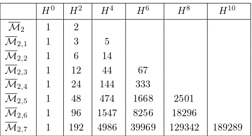
In Table 1 we present the nonequivariant information (remember that all co-homology is Tate) in the form of Betti numbers of M2,n for alln≤7. Notice
that the table only contains as many numbers as we need to be able to fill in the missing ones using Poincar´e duality. These results agree with Table 2 of ordinary Euler characteristics forM2,n forn≤6 found in [4].
Table 1. Dimensions ofHi(
M2,n⊗C,Q) forn≤7.
H0 H2 H4 H6 H8 H10
M2 1 2
M2,1 1 3 5 M2,2 1 6 14
M2,3 1 12 44 67 M2,4 1 24 144 333
M2,5 1 48 474 1668 2501 M2,6 1 96 1547 8256 18296
M2,7 1 192 4986 39969 129342 189289
The theorem used above also gives the corresponding results forM2,nforn≤7,
which we will present in terms of local systemsVλdefined as above, but starting
from V:=R1π
∗Q. See [14, Section 8] for the results on ec(M2⊗C,Vλ), for
Theorem 11.6. The Hodge Euler characteristics of the local systems Vλ on
M′
2:=M2⊗Cof weight 4or 6 are equal to
ec(M′2,V(4,0)) =0, ec(M′2,V(3,1)) =L2−1, ec(M2′,V(2,2)) =−L4,
ec(M′2,V(6,0)) =−1, ec(M′2,V(5,1)) =L2−L−1,
ec(M′2,V(4,2)) =L3, ec(M′2,V(3,3)) =−L−1.
12. Appendix: Introducing bi,ci and ri
This section will give an interpretation of the information carried by the ug’s.
It will be in terms of counts of hyperelliptic curves together with prescribed inverse images of points onP1 under their unique degree 2 morphism.
Definition 12.1. LetCϕ be a curve defined overktogether with a separable
degree 2 morphismϕoverkfromC toP1. We then define bi(Cϕ) :=|{α∈A(i) :|ϕ−1(α)|= 2, ϕ−1(α)⊆C(ki)}|,
ci(Cϕ) :=|{α∈A(i) :|ϕ−1(α)|= 2, ϕ−1(α)*C(ki)}|
and putri(Cϕ) :=bi(Cϕ) +ci(Cϕ).
The number of ramification points off that lie inA(i) is then equal to|A(i)| − ri(Cϕ).Letλidenote the partition oficonsisting of one element. We then find
that
|Cϕ(λi)|=|A(i)|+bi(Cϕ)−ci(Cϕ) +
(
2ci/2(Cϕ) ifiis even;
0 ifiis odd.
and thus
an(Cϕ) =
X
i|n: 2i∤n
ci(Cϕ)−bi(Cϕ)+
X
i:2i|n
−bi(Cϕ)−ci(Cϕ).
Definition 12.2. For partitionsµandν,g≥2 and odd characteristic, define
bµcν|g :=
X
[Cf]∈Hg(k)/∼=k
1 |Autk(Cf)|
l(µ)
Y
i=1
bi(Cf)µi l(ν)
Y
j=1
cj(Cf)νj.
The number|µ|+|ν| will be called the weight of this expression.
Remark 12.3. We can, in the obvious way, also define aλbµcν|g, but from
the relation between ai(Cf), bi(Cf) andci(Cf) we see that this gives no new
phenomena.
Directly from the definitions we get the following lemma.
Lemma 12.4. Let the characteristic be odd and letf be an element of Pg. We then have
bi(Cf) = 1
2
X
α∈A(i)
χ2,i f(α)
2
and
If the characteristic is odd we then use the same arguments as in Section 3 to conclude that
Note that this expression is defined for all g ≥ −1. It can be decomposed in terms of ug’s (that is, we can find a result corresponding to Lemma 3.8) for
tuples (n;r)∈ Nmsuch that
(12.1) |n| ≤ |µ|+|ν|.
Remark 12.5. The corresponding results clearly hold for elements (h, f) in Pg in even characteristic and the decomposition of bµcν|g is independent of
characteristic.
Example 12.6. For eachN we have the decomposition:
b[N]|g=
they are always equal to 0.
Lemma 12.8. For eachN, the following information is equivalent:
(1) all ug’s of degree at mostN;
(2) all bµcν|g of weight at mostN.
Proof: From property (12.1) of the decomposition of bµcν|g into ug’s we
directly find that if we know (1) we can compute (2). For the other direction we note on the one hand that
If we on the other hand decompose (12.2) intoug’s we find that there is a unique
ug of degreeS. The corresponding pair (n;r) contains, for eachi, preciselysi
entries of the formi1 andt
i entries of the formi2. Everyug of degree S can
be created in this way and hence if we know (2) we can compute (1).
Remark 12.9. From the definitions ofai(Cf) andri(Cf) we see that knowing
(1) and (2) in Lemma 12.8 is also equivalent to knowing (3) allaλrξ|g of weight at mostN,
whereaλrξ|g is defined in the obvious way. Moreover,aλrξ|g= 0 if|λ|is odd.
13. Appendix: The stable part of the counts
Remark 13.1. All results in this section are independent of characteristic.
Definition 13.2 ([8, Def. 1.2.1, 1.2.2]). Let F be a constructible (ℓ-adic) sheaf on a scheme X of finite type over Z. The sheaf F is said to be pure
of weight m if, for every closed point x in X and eigenvalue αof Frobenius F (relative to k = k(x)) acting on Fx¯, α is an algebraic integer of weight equal tom, i.e., such that all its conjugates have absolute value equal toqm/2. The sheaf F is said to be mixed of weight ≤ m if there exists a filtration 0 =F−1⊂ F0 ⊂. . .⊂ Fm=F of constructible subsheaves such that, for all
j,Fj/Fj−1is pure of weightj.
Theorem 13.3 ([8, Cor. 3.3.3, 3.3.4]). Let X −→f Zbe a scheme of finite type, and F a constructible sheaf mixed of weight ≤ m. Then Rif!
F is mixed of weight ≤m+i. Thus, for every finite fieldk, there is a filtration0 =W−1⊂ W0 ⊂. . .⊂Wi+m=Hci(X¯k,F) ofGal(¯k/k)-representations such that, for all
j,Wj/Wj−1 is pure of weightj.
Definition13.4. LetK0(Galk) be the Grothendieck group of Gal(¯
k/k)-repre-sentations. In this category, and with the notation of Theorem 13.3, we have [Hi
c(X¯k,F)] =
Pi+m
j=0[Wj/Wj−1]. For anyw≥0, let us define [Hci(X¯k,F)]w:=
Pi+m
j=w[Wj/Wj−1] andewc(X¯k,F) :=
P
i≥0(−1)i[Hci(X¯k,F)]win K0(Galk). We
make the corresponding definition ofewc(XQ,F) inK0(GalQ).
Recall the definition in Section 11.1, for a primeℓ∤q, of theℓ-adic local system VλonHg. Ifτis the canonical morphism fromHg⊗k¯toHg, we putV′λ=τ∗Vλ.
This is a constructible sheaf pure of weight|λ|.
In this section we will see that ifgandware large enough we can compute the trace of Frobenius onewc(Hg⊗¯k,Vλ), which by definition (cf. Section 2 in [3])
is equal toewc(Hg,V′λ). We first make the connection toSn-equivariant counts
of points ofHg,nexplicit.
Lemma 13.5. Let the symmetric polynomial s<λ> be the Schur polynomial in the symplectic case (see [11, A.45]), and pλ the power sum. If s<λ> =
P
|µ|≤|λ|mµpµ then
(13.1) Tr F,ec(Hg⊗¯k,V′λ)
= X
|µ|≤|λ|
mµq 1