El e c t ro n ic
Jo ur n
a l o
f P
r o b
a b i l i t y Vol. 12 (2007), Paper no. 18, pages 516–573.
Journal URL
http://www.math.washington.edu/~ejpecp/
Intermittency on catalysts: symmetric exclusion
∗J¨urgen G¨artner Institut f¨ur Mathematik Technische Universit¨at Berlin
Straße des 17. Juni 136 D-10623 Berlin, Germany
Frank den Hollander Mathematical Institute Leiden University, P.O. Box 9512 2300 RA Leiden, The Netherlands
and EURANDOM, P.O. Box 513 5600 MB Eindhoven, The Netherlands
Gregory Maillard Institut de Math´ematiques ´
Ecole Polytechnique F´ed´erale de Lausanne CH-1015 Lausanne, Switzerland
Abstract
We continue our study of intermittency for the parabolic Anderson equation ∂u/∂t = κ∆u+ξu, whereu: Zd×[0,∞)→R,κis the diffusion constant, ∆ is the discrete Laplacian, and ξ: Zd ×[0,∞) → R is a space-time random medium. The solution of the equation describes the evolution of a “reactant”uunder the influence of a “catalyst”ξ.
In this paper we focus on the case whereξis exclusion with a symmetric random walk tran-sition kernel, starting from equilibrium with density ρ∈ (0,1). We consider the annealed
∗The research in this paper was partially supported by the DFG Research Group 718 “Analysis and Stochastics
Lyapunov exponents, i.e., the exponential growth rates of the successive moments ofu. We show that these exponents are trivial when the random walk is recurrent, but display an interesting dependence on the diffusion constantκwhen the random walk is transient, with qualitatively different behavior in different dimensions. Special attention is given to the asymptotics of the exponents for κ→ ∞, which is controlled by moderate deviations ofξ requiring a delicate expansion argument.
In G¨artner and den Hollander (10) the case whereξ is a Poisson field of independent (sim-ple) random walks was studied. The two cases show interesting differences and similarities. Throughout the paper, a comparison of the two cases plays a crucial role.
Key words: Parabolic Anderson model, catalytic random medium, exclusion process, Lya-punov exponents, intermittency, large deviations, graphical representation.
1
Introduction and main results
1.1 Model
The parabolic Anderson equation is the partial differential equation
∂
∂tu(x, t) =κ∆u(x, t) +ξ(x, t)u(x, t), x∈Z
d, t≥0. (1.1.1)
Here, the u-field is R-valued, κ ∈ [0,∞) is the diffusion constant, ∆ is the discrete Laplacian,
acting on uas
∆u(x, t) = X
y∈Zd ky−xk=1
[u(y, t)−u(x, t)] (1.1.2)
(k · k is the Euclidian norm), while
ξ ={ξ(x, t) : x∈Zd, t≥0} (1.1.3)
is an R-valued random field that evolves with time and that drives the equation. As initial
condition for (1.1.1) we take
u(·,0)≡1. (1.1.4)
Equation (1.1.1) is a discrete heat equation with theξ-field playing the role of a source. What makes (1.1.1) particularly interesting is that the two terms in the right-hand sidecompete with each other: the diffusion induced by ∆ tends to make u flat, while the branching induced by
ξ tends to make u irregular. Intermittency means that for large t the branching dominates, i.e., the u-field develops sparse high peaks in such a way that u and its moments are each dominated by their own collection of peaks (see G¨artner and K¨onig (11), Section 1.3, and den Hollander (10), Section 1.2). In the quenched situation this geometric picture of intermittency is well understood for several classes of time-independent random potentials ξ (see Sznitman (21) for Poisson clouds and G¨artner, K¨onig and Molchanov (12) for i.i.d. potentials with double-exponential and heavier upper tails). For time-dependent random potentials ξ, however, such results are not yet available. Instead one restricts attention to understanding the phenomenon of intermittency indirectly by comparing the successive annealed Lyapunov exponents
λp= lim t→∞
1
t loghu(0, t)
pi1/p, p= 1,2, . . . (1.1.5)
One says that the solutionu is p-intermittent if thestrict inequality
λp > λp−1 (1.1.6)
holds. For a geometric interpretation of this definition, see (11), Section 1.3.
In their fundamental paper (3), Carmona and Molchanov succeeded to investigate the annealed Lyapunov exponents and to draw the qualitative picture of intermittency for potentials of the form
ξ(x, t) = ˙Wx(t), (1.1.7)
where{Wx, x∈Zd} denotes a collection of independent Brownian motions. (In this important
that ford= 1,2 intermittency of all orders is present for allκ, whereas ford≥3p-intermittency holds if and only if the diffusion constant κ is smaller than a critical threshold κ∗p tending to infinity as p → ∞. They also studied the asymptotics of the quenched Lyapunov exponent in the limit asκ↓0, which turns out to be singular. Subsequently, the latter was more thoroughly investigated in papers by Carmona, Molchanov and Viens (4), Carmona, Koralov and Molchanov (2), and Cranston, Mountford and Shiga (6), (7).
In the present paper we study a different model, describing the spatial evolution of moving reactants under the influence of moving catalysts. In this model, the potential has the form
ξ(x, t) =X
k
δYk(t)(x) (1.1.8)
with {Yk, k ∈ N} a collection of catalyst particles performing a space-time homogeneous
re-versible particle dynamics with hard core repulsion, and u(x, t) describes the concentration of the reactant particles given the motion of the catalyst particles. We will see later that the study of the annealed Lyapunov exponents leads todifferent dimension effects and requires the development ofdifferent techniques than in the white noise case (1.1.7). Indeed, because of the non-Gaussian nature and the non-independent spatial structure of the potential, it is far from obvious how to tackle the computation of Lyapunov exponents.
Let us describe our model in more detail. We consider the case whereξ isSymmetric Exclusion (SE), i.e.,ξ takes values in{0,1}Zd×[0,∞), where ξ(x, t) = 1 means that there is a particle at
x at timet and ξ(x, t) = 0 means that there is none, and particles move around according to a symmetric random walk transition kernel. We chooseξ(·,0) according to the Bernoulli product measure with densityρ∈(0,1), i.e., initially each site has a particle with probability ρ and no particle with probability 1−ρ, independently for different sites. For this choice, the ξ-field is stationary in time.
One interpretation of (1.1.1) and (1.1.4) comes from population dynamics. Consider a spatially homogeneous system of two types of particles, A(catalyst) andB (reactant), subject to:
(i) A-particles behave autonomously, according to a prescribed stationary dynamics, with densityρ;
(ii) B-particles perform independent random walks with diffusion constant κ and split into two at a rate that is equal to the number ofA-particles present at the same location;
(iii) the initial density of B-particles is 1.
Then
u(x, t) = the average number ofB-particles at site x at timet
conditioned on the evolution of the A-particles. (1.1.9)
It is possible to add that B-particles die at rate δ ∈ (0,∞). This amounts to the trivial transformationu(x, t)→u(x, t)e−δt.
1.2 SE, Lyapunov exponents and comparison with IRW
Throughout the paper, we abbreviate Ω ={0,1}Zd
(endowed with the product topology), and we let p:Zd×Zd→[0,1] be the transition kernel of an irreducible random walk,
p(x, y) =p(0, y−x)≥0 ∀x, y∈Zd, X
y∈Zd
p(x, y) = 1 ∀x∈Zd,
p(x, x) = 0 ∀x∈Zd, p(·,·) generates Zd,
(1.2.1)
that is assumed to besymmetric,
p(x, y) =p(y, x) ∀x, y∈Zd. (1.2.2)
A special case is simple random walk
p(x, y) =
( 1
2d ifkx−yk= 1,
0 otherwise. (1.2.3)
The exclusion process ξ is the Markov process on Ω whose generator L acts on cylindrical functionsf as (see Liggett (19), Chapter VIII)
(Lf)(η) = X
x,y∈Zd
p(x, y)η(x)[1−η(y)] [f(ηx,y)−f(η)] = X
{x,y}⊂Zd
p(x, y) [f(ηx,y)−f(η)],
(1.2.4) where the latter sum runs over unoriented bonds{x, y}between any pair of sites x, y∈Zd, and
ηx,y(z) =
η(z) ifz6=x, y, η(y) ifz=x, η(x) ifz=y.
(1.2.5)
The first equality in (1.2.4) says that a particle at site x jumps to a vacancy at site y at rate
p(x, y), the second equality says that the states of x and y are interchanged along the bond {x, y} at rate p(x, y). For ρ∈[0,1], let νρ be the Bernoulli product measure on Ω with density
ρ. This is an invariant measure for SE. Under (1.2.1–1.2.2), (νρ)ρ∈[0,1] are the only extremal
equilibria (see Liggett (19), Chapter VIII, Theorem 1.44). We denote byPη the law ofξ starting
from η∈Ω and writePνρ =RΩνρ(dη)Pη.
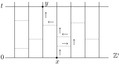
In the graphical representation of SE, space is drawn sidewards, time is drawn upwards, and for each pair of sites x, y ∈ Zd links are drawn between x and y at Poisson rate p(x, y). The configuration at timetis obtained from the one at time 0 by transporting the local states along paths that move upwards with time and sidewards along links (see Fig. 1).
We will frequently use the following property, which is immediate from the graphical represen-tation:
Eη(ξ(y, t)) = X
x∈Zd
η(x)pt(x, y), η∈Ω, y∈Zd, t≥0. (1.2.6)
Similar expressions hold for higher order correlations. Here, pt(x, y) is the probability that
The graphical representation shows that the evolution is invariant under time reversal and, in particular, the equilibria (νρ)ρ∈[0,1] are reversible. This fact will turn out to be very important
later on.
x y
0
t
→ ← ←
↑ ↑ ↑ ↑
r r
Zd
Fig. 1: Graphical representation. The dashed lines are links. The arrows represent a path from (x,0) to (y, t).
By the Feynman-Kac formula, the solution of (1.1.1) and (1.1.4) reads
u(x, t) =Ex
exp
Z t
0
ds ξ(Xκ(s), t−s)
, (1.2.7)
where Xκ is simple random walk on Zd with step rate 2dκ and Ex denotes expectation with
respect toXκ givenXκ(0) =x. We will often write ξ
t(x) and Xtκ instead of ξ(x, t) and Xκ(t),
respectively.
Forp∈N and t >0, define
Λp(t) =
1
ptlogEνρ(u(0, t)
p). (1.2.8)
Then
Λp(t) =
1
ptlogEνρ
E0,...,0
exp
Z t
0
ds
p
X
q=1
ξ Xqκ(s), s
, (1.2.9)
where Xqκ, q = 1, . . . , p, are p independent copies of Xκ, E0,...,0 denotes expectation w.r.t.
Xqκ, q = 1, . . . , p, given X1κ(0) = · · · = Xpκ(0) = 0, and the time argument t−s in (1.2.7) is replaced bys in (1.2.9) via the reversibility ofξ starting fromνρ. If the last quantity admits a
limit ast→ ∞, then we define
λp = lim
t→∞Λp(t) (1.2.10)
to be thep-th annealed Lyapunov exponent.
From H¨older’s inequality applied to (1.2.8) it follows that Λp(t) ≥ Λp−1(t) for all t > 0 and
p ∈ N\ {1}. Hence λp ≥ λp−1 for all p ∈ N\ {1}. As before, we say that the system is p
-intermittent if λp > λp−1. In the latter case the system is q-intermittent for all q > p as well
(cf. G¨artner and Molchanov (13), Section 1.1). We say that the system is intermittent if it is
p-intermittent for all p∈N\ {1}.
Let (˜ξt)t≥0 be the process of Independent Random Walks (IRW) with step rate 1, transition
kernel p(·,·) and state space Ω =e NZd
0 with N0 = N∪ {0}. Let EIRWη denote expectation w.r.t.
(˜ξt)t≥0 starting from ˜ξ0 =η ∈ Ω, and writeEIRWνρ =
R
Ωνρ(dη)E IRW
η . Throughout the paper we
Proposition 1.2.1. For any K: Zd×[0,∞)→R such that either K ≥0 or K ≤0, any t≥0
such thatPz∈Zd
Rt
0 ds|K(z, s)|<∞ and any η∈Ω,
Eη exp
" X
z∈Zd
Z t
0
ds K(z, s)ξs(z)
#!
≤EIRW
η exp
" X
z∈Zd
Z t
0
ds K(z, s) ˜ξs(z)
#!
. (1.2.11)
This powerful inequality will allow us to obtain bounds that are more easily computable.
1.3 Main theorems
Our first result is standard and states that the Lyapunov exponents exist and behave nicely as a function ofκ. We write λp(κ) to exhibit the dependence onκ, suppressingdand ρ.
Theorem 1.3.1. Let d≥1, ρ∈(0,1) and p∈N.
(i) For all κ∈[0,∞), the limit in (1.2.10)exists and is finite. (ii) On [0,∞), κ→λp(κ) is continuous, non-increasing and convex.
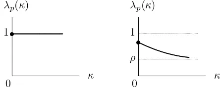
Our second result states that the Lyapunov exponents are trivial for recurrent random walk but are non-trivial for transient random walk (see Fig. 2), without any further restriction onp(·,·).
Theorem 1.3.2. Let d≥1, ρ∈(0,1) and p∈N.
(i) Ifp(·,·) is recurrent, then λp(κ) = 1 for allκ∈[0,∞).
(ii) Ifp(·,·) is transient, then ρ < λp(κ)<1 for all κ∈[0,∞). Moreover, κ7→λp(κ) is strictly
decreasing withlimκ→∞λp(κ) =ρ.
0 1
κ λp(κ)
0 1
ρ
κ λp(κ)
s
s
Fig. 2: Qualitative picture ofκ7→λp(κ) for recurrent, respectively,
transient random walk.
Our third result shows that for transient random walk the system is intermittent for small κ.
Theorem 1.3.3. Let d≥1 and ρ ∈ (0,1). If p(·,·) is transient, then there exists κ0 ∈(0,∞]
such thatp7→λp(κ) is strictly increasing forκ∈[0, κ0).
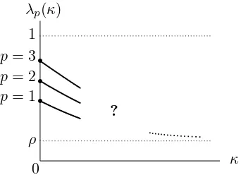
Our fourth and final result identifies the behavior of the Lyapunov exponents forlarge κ when
d≥4 and p(·,·) is simple random walk (see Fig. 3).
Theorem 1.3.4. Assume (1.2.3). Let d≥4,ρ∈(0,1) and p∈N . Then
lim
κ→∞κ[λp(κ)−ρ] =
1
2dρ(1−ρ)Gd (1.3.1)
0
ρ
1
r
r
r
p= 3
p= 2
p= 1
?
κ λp(κ)
Fig. 3: Qualitative picture ofκ7→λp(κ) forp= 1,2,3 for simple
random walk ind≥4. The dotted line moving down represents the asymptotics given by the r.h.s. of (1.3.1).
1.4 Discussion
Theorem 1.3.1 gives general properties that need no further comment. We will see that they in fact hold forany stationary, reversible and bounded ξ.
The intuition behind Theorem 1.3.2 is the following. If the catalyst is driven by a recurrent random walk, then it suffers from “traffic jams”, i.e., with not too small a probability there is a large region around the origin that the catalyst fully occupies for a long time. Since with not too small a probability the simple random walk (driving the reactant) can stay inside this large region for the same amount of time, the average growth rate of the reactant at the origin is maximal. This phenomenon may be expressed by saying that for recurrent random walk clumping of the catalyst dominates the growth of the moments. For transient random walk, on the other hand, clumping of the catalyst is present (the growth rate of the reactant is > ρ), but it is not dominant (the growth rate of the reactant is <1). As the diffusion constant κ of the reactant increases, the effect of the clumping of the catalyst gradually diminishes and the growth rate of the reactant gradually decreases to the density of the catalyst.
Theorem 1.3.3 shows that if the reactant stands still and the catalyst is driven by a transient random walk, then the system is intermittent. Apparently, the successive moments of the reac-tant, which are equal to the exponential moments of the occupation time of the origin by the catalyst (take (1.2.7) withκ= 0), are sensitive tosuccessive degrees of clumping. By continuity, intermittency persists for small κ.
Theorem 1.3.4 shows that, when the catalyst is driven by simple random walk, all Lyapunov exponents decay toρ asκ→ ∞ in the same manner whend≥4. The cased= 3 remains open. We conjecture:
Conjecture 1.4.1. Assume (1.2.3). Let d= 3, ρ∈(0,1) andp∈N. Then
lim
κ→∞κ[λp(κ)−ρ] =
1
2dρ(1−ρ)Gd+ [2dρ(1−ρ)p]
2P (1.4.1)
with
P = sup
f∈H1(R3)
kfk2=1
(−∆R3)−1/2 f2 2
2− k∇R3fk 2 2
where ∇R3 and ∆R3 are the continuous gradient and Laplacian, k · k2 is the L2(R3)-norm,
H1(R3) ={f: R3→R: f,∇
R3f ∈L2(R3)}, and
(−∆R3)−1/2 f2 2
2=
Z
R3
dx f2(x)
Z
R3
dy f2(y) 1
4πkx−yk. (1.4.3)
In Section 1.5 we will explain how this conjecture arises in analogy with the case of IRW studied in G¨artner and den Hollander (10). If Conjecture 1.4.1 holds true, then in d= 3 intermittency persists for largeκ. It would still remain open whether the same is true ford≥4. To decide the latter, we need a finer asymptotics ford≥4. A large diffusion constant of the reactant hampers the localization of u around the regions where the catalyst clumps, but it is not a priori clear whether this is able to destroy intermittency ford≥4.
We further conjecture:
Conjecture 1.4.2. Ind= 3, the system is intermittent for allκ∈[0,∞).
Conjecture 1.4.3. Ind≥4, there exists a strictly increasing sequence 0< κ2 < κ3 < . . . such
that forp= 2,3, . . . the system is p-intermittent if and only if κ∈[0, κp).
In words, we conjecture that ind= 3 the curves in Fig. 3 never merge, whereas for d≥4 the curves merge successively.
Let us briefly compare our results for the simple symmetric exclusion dynamics with those of the IRW dynamics studied in (10). If the catalysts are moving freely, then they can accumulate with a not too small probability at single lattice sites. This leads to a double-exponential growth of the moments ford= 1,2. The same is true ford≥3 for certain choices of the model parameters (‘strongly catalytic regime’). Otherwise the annealed Lyapunov exponents are finite (‘weakly catalytic regime’). For our exclusion dynamics, there can be at most one catalytic particle per site, leading to the degenerate behavior for d = 1,2 (i.e., the recurrent case) as stated in Theorem 1.3.2(i). Ford≥3, the largeκbehavior of the annealed Lyapunov exponents turns out to be the same as in the weakly catalytic regime for IRW. The proof of Theorem 1.3.4 will be carried out in Section 4 essentially by ‘reducing’ its assertion to the corresponding statement in (10), as will be explained in Section 1.5. The reduction is highly technical, but seems to indicate a degree of ‘universality’ in the behavior of a larger class of models.
Finally, let us explain why we cannot proceed directly along the lines of (10). In that paper, the key is a Feynman-Kac representation of the moments. For the first moment, for instance, we have
hu(0, t)i=eνtE0
exp
ν
Z t
0
w(X(s), s)ds
, (1.4.4)
where X is simple random walk on Zd with generator κ∆ starting from the origin, ν is the
density of the catalysts, andw denotes the solution of the random Cauchy problem
∂
∂tw(x, t) =̺∆w(x, t) +δX(t)(x){w(x, t) + 1}, w(·,0) ≡0, (1.4.5)
with ̺ the diffusion constant of the catalysts. In the weakly catalytic regime, for large κ, we may combine (1.4.4) with the approximation
w(X(s), s) ≈
Z s
0
wherept(x, y) is the transition kernel of the catalysts. Observe that w(X(s), s) depends on the
full past of X up to time s. The entire proof in (10) is based on formula (1.4.4). But for our exclusion dynamics there isno such formula for the moments.
1.5 Heuristics behind Theorem 1.3.4 and Conjecture 1.4.1
The heuristics behind Theorem 1.3.4 and Conjecture 1.4.1 is the following. Consider the case
p= 1. Scaling time byκ in (1.2.9), we haveλ1(κ) =κλ∗1(κ) with
For largeκ, theξ-field in (1.5.1) evolves slowly and therefore does not manage to cooperate with theX-process in determining the growth rate. Also, the prefactor 1/κin the exponent is small. As a result, the expectation over theξ-field can be computed via aGaussian approximation that becomes sharp in the limit asκ→ ∞, i.e., (In essence, what happens here is that the asymptotics for κ → ∞ is driven by moderate deviations of theξ-field, which fall in the Gaussian regime.) The exponent in the r.h.s. of (1.5.3) equals
where the first equality uses the stationarity ofξ, the third equality uses (1.2.6) from the graphical representation, and the fourth equality uses thatνρis Bernoulli. Substituting (1.5.5) into (1.5.4),
we get that the r.h.s. of (1.5.3) equals
This is precisely the integral that was investigated in G¨artner and den Hollander (10) (see Sections 5–8 and equations (1.5.4–1.5.11) of that paper and 1.4.4-1.4.5). Therefore the limit
lim
κ→∞κ[λ1(κ)−ρ] = limκ→∞κ
2 lim
t→∞ h
Λ∗1(κ;t)− ρ
κ
i
= lim
κ→∞κ
2 lim
t→∞(1.5.6) (1.5.7)
can be read off from (10) and yields (1.3.1) ford≥4 and (1.4.1) ford= 3. A similar heuristics applies forp >1.
The r.h.s. of (1.3.1), which is valid ford≥4, is obtained from the above computations by moving the expectation in (1.5.6) into the exponent. Indeed,
E0
pu−s
κ (X(s), X(u))
= X
x,y∈Zd
p2ds(0, x)p2d(u−s)(x, y)pu−s
κ (x, y) =p2d(u−s)(1+
1 2dκ)(0,0)
(1.5.8) and hence
Z t
0
ds
Z t
s
du E0
pu−s
κ (X(s), X(u))
=
Z t
0
ds
Z t−s
0
dv p2dv(1+ 1
2dκ)(0,0) ∼t
1
2d(1 +2dκ1 )Gd. (1.5.9) Thus we see that the result in Theorem 1.3.4 comes from asecond order asymptotics onξ and a first order asymptotics on X in the limit as κ→ ∞. Despite this simple fact, it turns out to be hard to make the above heuristics rigorous. Ford= 3, on the other hand, we expect the first order asymptotics onX to fail, leading to the more complicated behavior in (1.4.1).
Remark 1: In (1.1.1), the ξ-field may be multiplied by a coupling constant γ ∈(0,∞). This produces no change in Theorems 1.3.1, 1.3.2(i) and 1.3.3. In Theorem 1.3.2(ii), (ρ,1) becomes (γρ, γ), while in the r.h.s. of Theorem 1.3.4 and Conjecture 1.4.1, ρ(1−ρ) gets multiplied by
γ2. Similarly, if the simple random walk in Theorem 1.3.4 is replaced by a random walk with transition kernel p(·,·) satisfying (1.2.1–1.2.2), then we expect that in (1.3.1) and (1.4.1) Gd
becomes the Green function at the origin of this random walk and a factor 1/σ4 appears in front
of the last term in the r.h.s. of (1.4.1) withσ2 the variance of p(·,·).
Remark 2: In G¨artner and den Hollander (10) the catalyst was γ times a Poisson field with density ρ of independent simple random walks stepping at rate 2dθ, whereγ, ρ, θ ∈ (0,∞) are parameters. It was found that the Lyapunov exponents are infinite in d= 1,2 for all p and in
d≥3 for p≥2dθ/γGd, irrespective ofκ and ρ. In d≥3 for p < 2dθ/γGd, on the other hand,
the Lyapunov exponents are finite for allκ, and exhibit a dichotomy similar to the one expressed by Theorem 1.3.4 and Conjecture 1.4.1. Apparently, in this regime the two types of catalyst are qualitatively similar. Remarkably, the same asymptotic behavior for large κ was found (with
ργ2replacingρ(1−ρ) in (1.3.1)), and thesame variational formula as in (1.4.2) was seen to play
a central role ind= 3. [Note: In (10) the symbolsν, ρ, Gd were used instead of ρ, θ, Gd/2d.]
1.6 Outline
In Section 2 we derive a variational formula forλpfrom which Theorem 1.3.1 follows immediately.
λp derived in Section 2, to prove Theorems 1.3.2 and 1.3.3. Here, the special properties of SE, in
particular, its space-time correlation structure expressed through the graphical representation (see Fig. 1), are crucial. These results hold for an arbitrary random walk subject to (1.2.1–1.2.2). Finally, in Section 4 we prove Theorem 1.3.4, which is restricted to simple random walk. The analysis consists of a long series of estimates, taking up more than half of the paper and, in essence, showing that the problem reduces to understanding the asymptotic behavior of (1.5.6). This reduction is important, because it explains why there is some degree ofuniversality in the behavior forκ→ ∞ under different types of catalysts: apparently, the Gaussian approximation and the two-point correlation function in space and time determine the asymptotics (recall the heuristic argument in Section 1.5). The main steps of this long proof are outlined in Section 4.2.
2
Lyapunov exponents: general properties
In this section we prove Theorem 1.3.1. In Section 2.1 we formulate a large deviation principle for the occupation time of the origin in SE due to Landim (18), which will be needed in Section 3.2. In Section 2.2 we extend the line of thought in (18) and derive a variational formula forλp
from which Theorem 1.3.1 will follow immediately.
2.1 Large deviations for the occupation time of the origin
Kipnis (17), building on techniques developed by Arratia (1), proved that the occupation time of the origin up to time t,
Tt=
Z t
0
ξ(0, s)ds, (2.1.1)
satisfies a strong law of large numbers and a central limit theorem. Landim (18) subsequently proved thatTt satisfies a large deviation principle, i.e.,
lim sup
t→∞
1
t logPνρ(Tt/t∈F)≤ − inf
α∈FΨd(α), F ⊆[0,1] closed,
lim inf
t→∞
1
t logPνρ(Tt/t∈G)≥ − inf
α∈GΨd(α), G⊆[0,1] open,
(2.1.2)
with the rate function Ψd: [0,1] → [0,∞) given by an associated Dirichlet form. This rate
function is continuous, for transient random walk kernelsp(·,·) it has a unique zero atρ, whereas for recurrent random walk kernels it vanishes identically.
2.2 Variational formula for λp(κ): proof of Theorem 1.3.1
Return to (1.2.9). In this section we show that, by considering ξ and Xκ
1, . . . , Xpκ as a joint
random process and exploiting the reversibility ofξ, we can use the spectral theorem to express the Lyapunov exponents in terms of a variational formula. From the latter it will follow that
κ7→λp(κ) is continuous, non-increasing and convex on [0,∞).
Define
and
V(η, x1, . . . , xp) = p
X
i=1
η(xi), η∈Ω, x1, . . . , xp∈Zd. (2.2.2)
Then we may write (1.2.9) as
Λp(t) =
1
ptlogEνρ,0,...,0
exp
Z t
0
V(Y(s))ds
. (2.2.3)
The random processY = (Y(t))t≥0 takes values in Ω×(Zd)p and has generator
Gκ =L+κ
p
X
i=1
∆i (2.2.4)
inL2(νρ⊗mp) (endowed with the inner product (·,·)), withL given by (1.2.4), ∆i the discrete
Laplacian acting on thei-th spatial coordinate, andm the counting measure onZd. Let
GκV =Gκ+V. (2.2.5)
By (1.2.2), this is aself-adjoint operator. Our claim is thatλpequals 1p times the upper boundary
of the spectrum of Gκ V.
Proposition 2.2.1. λp = 1pµp with µp = sup Sp (GκV).
Although this is a general fact, the proofs known to us (e.g. Carmona and Molchanov (3), Lemma III.1.1) do not work in our situation.
Proof. Let (Pt)t≥0 denote the semigroup generated byGκV.
Upper bound: Let Qtlogt = [−tlogt, tlogt]d∩Zd. By a standard large deviation estimate for
simple random walk, we have
Eν
ρ,0,...,0
exp
Z t
0
V(Y(s))ds
=Eνρ,0,...,0
exp
Z t
0
V(Y(s))ds
11{Xiκ(t)∈Qtlogtfori= 1, . . . , p}
+Rt
(2.2.6)
with limt→∞1tlogRt=−∞. Thus it suffices to focus on the term with the indicator.
Estimate, with the help of the spectral theorem (Kato (15), Section VI.5),
Eνρ,0,...,0
exp
Z t
0
V(Y(s))ds
11{Xiκ(t)∈Qtlogt fori= 1, . . . , p}
≤11(Qtlogt)p,Pt11(Q tlogt)p
=
Z
(−∞,µp]
eµtdkEµ11(Qtlogt)pk
2
L2(νρ⊗mp)
≤eµptk11
(Qtlogt)pk
2
L2(νρ⊗mp),
(2.2.7)
where11(Qtlogt)p is the indicator function of (Qtlogt)p ⊂(Zd)p and (Eµ)µ∈R denotes the spectral
family of orthogonal projection operators associated with Gκ
V. Since k11(Qtlogt)pk
2
|Qtlogt|p does not increase exponentially fast, it follows from (1.2.10), (2.2.3) and (2.2.6–2.2.7)
thatλp ≤ 1pµp.
Lower bound: For every δ >0 there exists anfδ∈L2(νρ⊗mp) such that
(Eµp−Eµp−δ)fδ6= 0 (2.2.8)
(see Kato (15), Section VI.2; the spectrum ofGκV coincides with the set ofµ’s for whichEµ+δ−
Eµ−δ 6= 0 for all δ > 0). Approximating fδ by bounded functions, we may without loss of
generality assume that 0≤fδ≤1. Similarly, approximatingfδby bounded functions with finite
support in the spatial variables, we may assume without loss of generality that there exists a finite Kδ ⊂Zd such that
0≤fδ ≤11(Kδ)p. (2.2.9)
First estimate
Eνρ,0,...,0
exp
Z t
0
V(Y(s))ds
≥ X
x1,...,xp∈Kδ
Eν
ρ,0,...,0
11{X1κ(1) =x1, . . . , Xpκ(1) =xp} exp
Z t
1
V(Y(s))ds
= X
x1,...,xp∈Kδ
pκ1(0, x1). . . pκ1(0, xp)Eνρ,x1,...,xp
exp
Z t−1
0
V(Y(s))ds
≥Cδp X
x1,...,xp∈Kδ
Eν
ρ,x1,...,xp
exp
Z t−1
0
V(Y(s))ds
,
(2.2.10)
where pκt(x, y) =Px(Xκ(t) =y) and Cδ = minx∈K
δp
κ
1(0, x) >0. The equality in (2.2.10) uses
the Markov property and the fact thatνρ is invariant for the SE-dynamics. Next estimate
r.h.s. (2.2.10)≥Cδp
Z
Ω
νρ(dη)
X
x1,...,xp∈Zd
fδ(η, x1, . . . , xp)
×Eη,x
1,...,xp
exp
Z t−1
0
V(Y(s))ds
fδ(Y(t−1))
=Cδp(fδ,Pt−1fδ)≥
Cδp
|Kδ|p
Z
(µp−δ,µp]
eµ(t−1)dkEµfδk2L2(νρ⊗mp)
≥Cδpe(µp−δ)(t−1)k(E
µp−Eµp−δ)fδk
2
L2(νρ⊗mp),
(2.2.11)
where the first inequality uses (2.2.9). Combine (2.2.10–2.2.11) with (2.2.8), and recall (2.2.3), to getλp≥ p1(µp−δ). Letδ ↓0, to obtain λp ≥ 1pµp.
The Rayleigh-Ritz formula for µp applied to Proposition 2.2.1 gives (recall (1.2.4), (2.2.2) and
(2.2.4–2.2.5)):
Proposition 2.2.2. For all p∈N,
λp =
1
pµp =
1
p kfk sup
L2 (νρ⊗mp)=1
with
(GκVf, f) =A1(f)−A2(f)−κA3(f), (2.2.13)
where
A1(f) = Z
Ω
νρ(dη)
X
z1,...,zp∈Zd
V(η;z1, . . . , zp)f(η, z1, . . . , zp)2,
A2(f) = Z
Ω
νρ(dη)
X
z1,...,zp∈Zd
1 2
X
{x,y}⊂Zd
p(x, y) [f(ηx,y, z1, . . . , zp)−f(η, z1, . . . , zp)]2,
A3(f) = Z
Ω
νρ(dη)
X
z1,...,zp∈Zd
1 2
p
X
i=1 X
yi∈Zd
kyi−zik=1
[f(η, z1, . . . , zp)|zi→yi−f(η, z1, . . . , zp)]
2,
(2.2.14)
and zi →yi means that the argumentzi is replaced by yi.
Remark 2.2.3. Propositions 2.2.1–2.2.2 are valid for general bounded measurable potentials V
instead of (2.2.2). The proof also works for modifications of the random walk Y for which a lower bound similar to that in the last two lines of (2.2.10) can be obtained. Such modifications will be used later in Sections4.5–4.6.
We are now ready to give the proof of Theorem 1.3.1.
Proof. The existence of λp was established in Proposition 2.2.1. By (2.2.13–2.2.14), the r.h.s.
of (2.2.12) is a supremum over functions that are linear and non-increasing inκ. Consequently,
κ 7→ λp(κ) is lower semi-continuous, convex and non-increasing on [0,∞) (and, hence, also
continuous).
The variational formula in Proposition 2.2.2 is useful to deduce qualitative properties of λp,
as demonstrated above. Unfortunately, it is not clear how to deduce from it more detailed information about the Lyapunov exponents. To achieve the latter, we resort in Sections 3 and 4 to different techniques, only occasionally making use of Proposition 2.2.2.
3
Lyapunov exponents: recurrent vs. transient random walk
In this section we prove Theorems 1.3.2 and 1.3.3. In Section 3.1 we consider recurrent random walk, in Section 3.2 transient random walk.
3.1 Recurrent random walk: proof of Theorem 1.3.2(i)
The key to the proof of Theorem 1.3.2(i) is the following.
Lemma 3.1.1. If p(·,·) is recurrent, then for any finite box Q⊂Zd,
lim
t→∞
1
tlogPνρ
Proof. In the spirit of Arratia (1), Section 3, we argue as follows. Let
HtQ=nx∈Zd: there is a path from (x,0) toQ×[0, t] in the graphical representationo.
(3.1.2)
x
0
t
[ ←− Q −→ ]
→ →
→
↑ ↑
↑
r
r
Zd
Fig. 4: A path from (x,0) toQ×[0, t] (recall Fig. 1).
Note that H0Q = Q and that t 7→ HtQ is non-decreasing. Denote by P and E, respectively, probability and expectation associated with the graphical representation. Then
Pν
ρ
ξ(x, s) = 1 ∀s∈[0, t]∀x∈Q= (P ⊗νρ)
HtQ ⊆ξ(0), (3.1.3)
whereξ(0) ={x ∈Zd: ξ(x,0) = 1}is the set of initial locations of the particles. Indeed, (3.1.3) holds because if ξ(x,0) = 0 for somex ∈HtQ, then this 0 will propagate into Qprior to time t
(see Fig. 4).
By Jensen’s inequality,
(P ⊗νρ)
HtQ ⊆ξ(0)=Eρ|HtQ|
≥ρE|HtQ|. (3.1.4)
Moreover,HtQ ⊆ ∪y∈QHt{y}, and hence
E|HtQ| ≤ |Q| E|Ht{0}|. (3.1.5)
Furthermore, we have
E|Ht{0}|=Ep(·,·)
0 Rt, (3.1.6)
whereRtis the range after timetof the random walk with transition kernelp(·,·) drivingξ and
Ep(·,·)
0 denotes expectation w.r.t. this random walk starting from 0. Indeed, by time reversal,
the probability that there is a path from (x,0) to {0} ×[0, t] in the graphical representation is equal to the probability that the random walk starting from 0 hitsx prior to time t. It follows from (3.1.3–3.1.6) that
1
t logPνρ
ξ(x, s) = 1 ∀s∈[0, t] ∀x∈Q≥ −|Q|log
1
ρ
1
tE
p(·,·)
0 Rt
. (3.1.7)
Finally, since limt→∞1tE0p(·,·)Rt= 0 whenp(·,·) is recurrent (see Spitzer (20), Chapter 1, Section
We are now ready to give the proof of Theorem 1.3.2(i).
Proof. Since p7→λp is non-decreasing and λp ≤1 for all p∈N, it suffices to give the proof for
p= 1. Forp= 1, (1.2.9) gives
Λ1(t) =
1
t logEνρ,0
exp
Z t
0
ξ(Xκ(s), s)ds
. (3.1.8)
By restricting Xκ to stay inside a finite box Q ⊂ Zd up to time t and requiring ξ to be 1
throughout this box up to timet, we obtain
Eν
ρ,0
exp
Z t
0
ξ(Xκ(s), s)ds
≥etPνρ
ξ(x, s) = 1 ∀s∈[0, t] ∀x∈QP0
Xκ(s)∈Q∀s∈[0, t].
(3.1.9)
For the second factor, we apply (3.1.1). For the third factor, we have
lim
t→∞
1
t logP0
Xκ(s)∈Q ∀s∈[0, t]=−λκ(Q) (3.1.10)
with λκ(Q) > 0 the principal Dirichlet eigenvalue on Q of −κ∆, the generator of the simple random walkXκ. Combining (3.1.1) and (3.1.8–3.1.10), we arrive at
λ1 = lim
t→∞Λ1(t)≥1−λ
κ(Q). (3.1.11)
Finally, let Q → Zd and use that limQ→
Zdλκ(Q) = 0 for any κ, to arrive at λ1 ≥ 1. Since,
trivially, λ1 ≤1, we get λ1 = 1.
3.2 Transient random walk: proof of Theorems 1.3.2(ii) and 1.3.3
Theorem 1.3.2(ii) is proved in Sections 3.2.1 and 3.2.3–3.2.5, Theorem 1.3.3 in Section 3.2.2. Throughout the present section we assume that the random walk kernelp(·,·) is transient.
3.2.1 Proof of the lower bound in Theorem 1.3.2(ii)
Proposition 3.2.1. λp(κ)> ρ for allκ∈[0,∞) and p∈N.
Proof. Since p 7→ λp(κ) is non-decreasing for all κ, it suffices to give the proof for p = 1. For
everyǫ >0 there exists a function φǫ:Zd→Rsuch that
X
x∈Zd
φǫ(x)2 = 1 and
X
x,y∈Zd
kx−yk=1
[φǫ(x)−φǫ(y)]2 ≤ǫ2. (3.2.1)
Let
fǫ(η, x) =
1 +ǫη(x)
[1 + (2ǫ+ǫ2)ρ]1/2 φǫ(x), η∈Ω, x∈Z
Then
kfǫk2L2(ν
ρ⊗m)=
Z
Ω
νρ(dη)
X
x∈Zd
[1 +ǫη(x)]2
1 + (2ǫ+ǫ2)ρφǫ(x)
2= X
x∈Zd
φǫ(x)2 = 1. (3.2.3)
Therefore we may usefǫ as a test function in (2.2.12) in Proposition 2.2.2. This gives
λ1 =µ1≥ 1
1 + (2ǫ+ǫ2)ρ(I−II−κ III) (3.2.4)
with
I =
Z
Ω
νρ(dη)
X
z∈Zd
η(z) [1 +ǫη(z)]2φǫ(z)2 = (1 + 2ǫ+ǫ2)ρ
X
z∈Zd
φǫ(z)2 = (1 + 2ǫ+ǫ2)ρ (3.2.5)
and
II =
Z
Ω
νρ(dη)
X
z∈Zd
1 4
X
x,y∈Zd
p(x, y)ǫ2[ηx,y(z)−η(z)]2φǫ(z)2
= 1 2
Z
Ω
νρ(dη)
X
x,y∈Zd
p(x, y)ǫ2[η(x)−η(y)]2φǫ(x)2
=ǫ2ρ(1−ρ) X
x,y∈Zd
x6=y
p(x, y)φǫ(x)2 ≤ǫ2ρ(1−ρ)
(3.2.6)
and
III = 1 2
Z
Ω
νρ(dη)
X
x,y∈Zd kx−yk=1
[1 +ǫη(x)]φǫ(x)−[1 +ǫη(y)]φǫ(y)
2
= 1 2
X
x,y∈Zd kx−yk=1
[1 + (2ǫ+ǫ2)ρ][φǫ(x)2+φǫ(y)2]−2(1 +ǫρ)2φǫ(x)φǫ(y)
= 1
2[1 + (2ǫ+ǫ
2)ρ] X
x,y∈Zd kx−yk=1
[φǫ(x)−φǫ(y)]2+ǫ2ρ(1−ρ)
X
x,y∈Zd kx−yk=1
φǫ(x)φǫ(y)
≤ 1
2[1 + (2ǫ+ǫ
2)ρ]ǫ2+ 2dǫ2ρ(1−ρ).
(3.2.7)
In the last line we use thatφǫ(x)φǫ(y)≤ 12φǫ(x)2+12φǫ(y)2. Combining (3.2.4–3.2.7), we find
λ1=µ1≥ρ
1 + 2ǫ+O(ǫ2)
1 + 2ǫρ+O(ǫ2). (3.2.8)
3.2.2 Proof of Theorem 1.3.3
Proof. It is enough to show that λ2(0)> λ1(0). Then, by continuity (recall Theorem 1.3.1(ii)),
there exists κ0 ∈(0,∞] such that λ2(κ) > λ1(κ) for all κ ∈ [0, κ0), after which the inequality
λp+1(κ) > λp(κ) for κ ∈ [0, κ0) and arbitrary p follows from general convexity arguments (see
G¨artner and Heydenreich (9), Lemma 3.1). Forκ= 0, (1.2.9) reduces to
Λp(t) = 1
ptlogEνρ
exp
p
Z t
0
ξ(0, s)ds
= 1
ptlogEνρ(exp [pTt]) (3.2.9)
(recall (2.1.1)). In order to compute λp(0) = limt→∞Λp(t), we may use the large deviation
principle for (Tt)t≥0 cited in Section 2.1 due to Landim (18). Indeed, by applying Varadhan’s
Lemma (see e.g. den Hollander (14), Theorem III.13) to (3.2.9), we get
λp(0) = 1
pαmax∈[0,1]
pα−Ψd(α)
(3.2.10)
with Ψdthe rate function introduced in (2.1.2). Since Ψdis continuous, (3.2.10) has at least one
maximizerαp:
λp(0) =αp−
1
pΨd(αp). (3.2.11)
By Proposition 3.2.1 for κ = 0, we have λp(0) > ρ. Hence αp > ρ (because Ψd(ρ) = 0). Since
p(·,·) is transient, it follows that Ψd(αp)>0. Therefore we get from (3.2.10–3.2.11) that
λp+1(0)≥
1
p+ 1[αp(p+ 1)−Ψd(αp)] =αp− 1
p+ 1Ψd(αp)> αp− 1
pΨd(αp) =λp(0). (3.2.12)
In particularλ2(0)> λ1(0), and so we are done.
3.2.3 Proof of the upper bound in Theorem 1.3.2(ii)
Proposition 3.2.2. λp(κ)<1 for allκ∈[0,∞) and p∈N.
Proof. By Theorem 1.3.3, which was proved in Section 3.2.2, we know thatp7→λp(0) is strictly
increasing. Since λp(0) ≤ 1 for all p ∈ N, it therefore follows that λp(0) < 1 for all p ∈ N.
Moreover, by Theorem 1.3.1(ii), which was proved in Section 2.2, we know that κ 7→ λp(κ) is
non-increasing. It therefore follows thatλp(κ)<1 for all κ∈[0,∞) andp∈N.
3.2.4 Proof of the asymptotics in Theorem 1.3.2(ii)
The proof of the next proposition is somewhat delicate.
Proof. We give the proof forp= 1. The generalization to arbitrarypis straightforward and will be explained at the end. We need a cubeQ= [−R, R]d∩Zdof length 2R, centered at the origin
and δ∈(0,1). Limits are taken in the order
t→ ∞, κ→ ∞, δ↓0, Q↑Zd. (3.2.13)
The proof proceeds in 4 steps, each containing a lemma.
Step 1: LetXκ,Qbe simple random walk onQobtained fromXκby suppressing jumps outside of
Q. Then (ξt, Xtκ,Q)t≥0 is a Markov process on Ω×Qwith self-adjoint generator inL2(νρ⊗mQ),
wheremQ is the counting measure onQ.
Lemma 3.2.4. For all Q finite (centered and cubic) and κ∈[0,∞),
Eνρ,0
exp
Z t
0
ds ξ(Xsκ, s)
≤eo(t)Eνρ,0
exp
Z t
0
ds ξ Xsκ,Q, s
, t→ ∞. (3.2.14)
Proof. We consider the partition of Zd into cubes Qz = 2Rz +Q, z ∈ Zd. The Lyapunov
exponentλ1(κ) associated with Xκ is given by the variational formula (2.2.12–2.2.14) forp= 1.
It can be estimated from above by splitting the sums over Zd in (2.2.14) into separate sums
over the individual cubes Qz and suppressing inA3(f) the summands on pairs of lattice sites
belonging to different cubes. The resulting expression is easily seen to coincide with the original variational expression (2.2.12), except that the supremum is restricted in addition to functions
f with spatial support contained in Q. But this is precisely the Lyapunov exponent λQ1(κ) associated withXκ,Q. Hence, λ1(κ)≤λQ1(κ), and this implies (3.2.14).
Step 2: For large κ the random walk Xκ,Q moves fast through the finite box Q and therefore
samples it in a way that is close to the uniform distribution.
Lemma 3.2.5. For all Q finite and δ ∈ (0,1), there exist ε = ε(κ, δ, Q) and N0 = N0(δ, ε),
satisfying limκ→∞ε(κ, δ, Q) = 0and limδ,ε↓0N0(δ, ε) =N0 >1, such that
Eν
ρ,0
exp
Z t
0
ds ξ Xsκ,Q, s
≤o(1) + exp1 +1 +ε 1−δ
δN0|Q|+
δ+ε
1−δ
(t+δ)
×Eν
ρ
exp
Z t+δ
0
ds 1
|Q|
X
y∈Q
ξ(y, s)
, t→ ∞.
(3.2.15)
Proof. We split time into intervals of length δ > 0. Let Ik be the indicator of the event that
ξ has a jump time in Q during the k-th time interval. If Ik = 0, then ξs = ξ(k−1)δ for all
s∈[(k−1)δ, kδ). Hence,
Z kδ
(k−1)δ
ds ξs Xsκ,Q
≤
Z kδ
(k−1)δ
ds ξ(k−1)δ Xsκ,Q+δIk (3.2.16)
and, consequently, we have for all x∈Zd and k= 1, . . . ,⌈t/δ⌉,
Ex
exp
Z δ
0
ds ξ(k−1)δ+s Xsκ,Q
≤eδIkE
x
exp
Z δ
0
ds η Xsκ,Q
where we abbreviateξ(k−1)δ =η. Next, we do a Taylor expansion and use the Markov property Therefore, by the Lebesgue dominated convergence theorem, we have
lim This implies that the expression in the exponent in the r.h.s. of (3.2.18) converges to
δ
uniformly in η ∈ Ω. Combining the latter with (3.2.18), we see that there exists some ε =
ε(κ, δ, Q), satisfying limκ→∞ε(κ, δ, Q) = 0, such that for all x∈Q, Next, similarly as in (3.2.16), we have
δ 1
Applying the Markov property toXκ,Q, and using (3.2.16) and (3.2.23-3.2.24), we find that
where Nt+δ is the total number of jumps that ξ makes inside Q up to timet+δ. The second
term in the r.h.s. of (3.2.25) equals the second term in the r.h.s. of (3.2.15). The first term will be negligible on an exponential scale forδ ↓0, because, as can be seen from the graphical representation,Nt+δ is stochastically smaller that the total number of jumps up to time t+δ of
a Poisson process with rate|Q∪∂Q|. Indeed, abbreviating
a=
1 + 1 +ε 1−δ
δ, b= δ+ε
1−δ, Mt+δ=
Z t+δ
0
ds 1
|Q|
X
y∈Q
ξs(y), (3.2.26)
we estimate, for each N,
r.h.s.(3.2.25) =Eν
ρ
eaNt+δ+b(t+δ)+Mt+δ
≤e(b+1)(t+δ)Eν
ρ
eaNt+δ1{N
t+δ≥N|Q|(t+δ)}
+e(aN|Q|+b)(t+δ)Eν
ρ e
Mt+δ.
(3.2.27)
ForN ≥N0 =N0(a, b), the first term tends to zero ast→ ∞and can be discarded. Hence
r.h.s.(3.2.25)≤e(aN0|Q|+b)(t+δ)E
νρ
ebMt+δ
, (3.2.28)
which is the desired bound in (3.2.15). Note that a↓ 0, b ↓ 1 as δ, ε ↓ 0 and hence N0(a, b) ↓
N0 >1.
Step 3: By combining Lemmas 3.2.4–3.2.5, we now know that for anyQfinite,
lim
κ→∞λ1(κ)≤tlim→∞
1
tlogEνρ exp
" Z t
0
ds 1
|Q|
X
y∈Q
ξs(y)
#!
, (3.2.29)
where we have taken the limits κ → ∞ and δ ↓ 0. According to Proposition 1.2.1 (with
K(z, s) = (1/|Q|)1Q(z)),
Eν
ρ exp
" Z t
0
ds 1
|Q|
X
y∈Q
ξs(y)
#!
≤EIRW
νρ exp
" Z t
0
ds 1
|Q|
X
y∈Q
˜
ξs(y)
#!
, (3.2.30)
where (˜ξt)t≥0 is the process of Independent Random Walks onZdwith step rate 1 and transition
kernelp(·,·), and EIRW
νρ =
R
Ωνρ(dη)EIRWη . The r.h.s. can be computed and estimated as follows.
Write
(∆(p)f)(x) = X
y∈Zd
p(x, y)[f(y)−f(x)], x∈Zd, (3.2.31)
to denote the generator of the random walk with step rate 1 and transition kernelp(·,·).
Lemma 3.2.6. For all Q finite,
r.h.s.(3.2.30)≤eρt exp
Z t
0
ds 1
|Q|
X
x∈Q
wQ(x, s)
where wQ: Zd×[0,∞)→R is the solution of the Cauchy problem
which has the representation
wQ(x, t) =ERW
x denotes the expectation w.r.t. to Y starting from Y0=x.
Proof. Let
By the Feynman-Kac formula,vQ(x, t) is the solution of the Cauchy problem
∂vQ
Then (3.2.38) can be rewritten as (3.2.33). Combining (3.2.36–3.2.37) and (3.2.39), we get
r.h.s.(3.2.30) =
where we use that νρ is the Bernoulli product measure with densityρ. Summing (3.2.33) over
Integrating (3.2.41) w.r.t. time, we get
X
x∈Zd
wQ(x, t) =
Z t
0
ds X
x∈Q
1 |Q|w
Q(x, s) +t. (3.2.42)
Combining (3.2.40) and(3.2.42), we get the claim.
Step 4: The proof is completed by showing the following:
Lemma 3.2.7.
lim
Q↑Zdtlim→∞
1
t
Z t
0
ds 1
|Q|
X
x∈Q
wQ(x, s) = 0. (3.2.43)
Proof. LetG denote the Green operator acting on functionsV: Zd→[0,∞) as
(GV)(x) = X
y∈Zd
G(x, y)V(y), x∈Zd, (3.2.44)
whereG(x, y) =R0∞dt pt(x, y) denotes the Green kernel on Zd. We have
G
1
|Q|1|Q|
∞
= sup
x∈Zd
X
y∈Q
G(x, y) 1
|Q|. (3.2.45)
The r.h.s. tends to zero asQ↑Zd, becauseG(x, y) tends to zero askx−yk → ∞. Hence Lemma
8.2.1 in G¨artner and den Hollander (10) can be applied to (3.2.34) for Qlarge enough, to yield
sup
x∈Zd
s≥0
wQ(x, s)≤ε(Q)↓0 as Q↑Zd, (3.2.46)
which proves (3.2.43).
Combine (3.2.29–3.2.30), (3.2.32) and (3.2.43) to get the claim in Proposition 3.2.3.
This completes the proof of Proposition 3.2.3 for p = 1. The generalization to arbitrary p is straightforward and runs as follows. Return to (1.2.9). Separate thepterms under the sum with the help of H¨older’s inequality with weights 1/p. Next, use (3.2.14) for each of the p factors, leading to 1plog of the r.h.s. of (3.2.14) with an extra factor pin the exponent. Then proceed as before, which leads to Lemma 3.2.6 but withwQ the solution of (3.2.33) with |Qp|1Q(x) between
braces. Then again proceed as before, which leads to (3.2.40) but with an extra factor pin the r.h.s. of (3.2.42). The latter gives a factor epρt replacing eρt in (3.2.32). Now use Lemma 3.2.7 to get the claim.
3.2.5 Proof of the strict monotonicity in Theorem 1.3.2(ii)
By Theorem 1.3.1(ii), κ7→λp(κ) is convex. Because of Proposition 3.2.1 and Proposition 3.2.3,
4
Lyapunov exponents: transient simple random walk
This section is devoted to the proof of Theorem 1.3.4, whered≥4 andp(·,·) is simple random walk given by (1.2.3), i.e.,ξis simple symmetric exclusion (SSE).The proof is long and technical, taking up more than half of the present paper. After a time scaling in Section 4.1, an outline of the proof will be given in Section 4.2. The proof for p= 1 will then be carried out in Sections 4.3–4.7. In Section 4.8, we will indicate how to extend the proof to arbitraryp.
4.1 Scaling
As before, we writeXκ
s, ξs(x) instead of Xκ(s), ξ(x, s). We abbreviate
1[κ] = 1 + 1
2dκ, (4.1.1)
and write{a, b} to denote the unoriented bond between nearest-neighbor sites a, b∈Zd (recall
(1.2.3)–(1.2.4)). Three parameters will be important: t, κ and T. We will take limits in the following order:
t→ ∞, κ→ ∞, T → ∞. (4.1.2)
Fort≥0, let
Zt= (ξt
κ, Xt) (4.1.3)
and denote by Pη,x the law of Z starting from Z0 = (η, x). Then Z = (Zt)t≥0 is a Markov
process on Ω×Zd with generator
A= 1
κL+ ∆ (4.1.4)
(acting on the Banach space of bounded continuous functions on Ω×Zd, equipped with the
supremum norm). AbbreviateXκ
t =Xκt,t≥0, whereX= (Xt)t≥0 is simple random walk with
step rate 2d, being independent of (ξt)t≥0. We therefore have
Eν
ρ,0
exp
Z t
0
ds ξs(Xsκ)
=Eν
ρ,0
exp
1
κ
Z κt
0
ds ξs κ(Xs)
. (4.1.5)
Define the scaled Lyapunov exponent (recall (1.2.9–1.2.10))
λ∗1(κ) = lim
t→∞Λ ∗
1(κ;t) with Λ∗1(κ;t) =
1
tlogEνρ,0
exp
1
κ
Z t
0
ds ξs κ(Xs)
. (4.1.6)
Thenλ1(κ) =κλ∗1(κ). Therefore, in what follows we will focus on the quantity
λ∗1(κ)−ρ
κ = limt→∞
1
t logEνρ,0
exp
1
κ
Z t
0
dsξs
κ(Xs)−ρ
(4.1.7)
and compute its asymptotic behavior for large κ. We must show that
lim
κ→∞2dκ 2hλ∗
1(κ)−
ρ κ
i
4.2 Outline
To prove (4.1.8), we have to study the asymptotics of the expectation on the r.h.s. of (4.1.7) as
t→ ∞ and κ→ ∞(in this order). This expectation has the form
(In fact, such a solution exists only after an appropriate regularization, which turns out to be asymptotically correct ford≥4 but not ford= 3.) Then the term in the exponent of (4.2.1) is a martingaleMt modulo a remainder that stays bounded ast→ ∞:
1
(Lemma 4.3.1(i) below). Hence, the asymptotic investigation of (4.2.1) reduces to the study of
Eν
is an exponential martingale (Lemma 4.3.1(iii) below) and r is close to 1. Hence, applying H¨older’s inequality, we may bound the expectation in the r.h.s. of (4.2.4) from above by
with 1/r+ 1/q= 1 (and q large). A reverse H¨older inequality shows that this is a lower bound for large negative q. Because of the structure of the expected result (coming from a linear approximation of the exponential), the choice of a large |q|does not hurt. (This is not true for the result in Conjecture 1.4.1 pertaining to d= 3.) Hence, the whole proof essentially reduces to the derivation of an appropriate upper bound for
Eν
with arbitrary α ∈ R (c.f. Proposition 4.4.1 below). A Taylor expansion up to second order
shows that
the Rayleigh-Ritz formula shows that, asymptotically as t→ ∞, the expectation in (4.2.7) gets larger when we replaceXs by 0. Using an explicit representation of ψ, we see that
X
for certain kernels Kdiag and Koff (Lemma 4.6.2 below). Substituting this into the previous
formulas and separating the “diagonal” term from the “off-diagonal” term by use of the Cauchy-Schwarz inequality, we finally see that the whole proof reduces to showing that
lim sup (Lemmas 4.6.3 and 4.6.4 below). To prove the latter statements, we use Jensen’s inequality to move the kernelsKdiag and Koff out of the exponents. Then we are left with the derivation of
upper bounds for terms of the form
Eν
(Lemmas 4.6.8 and 4.6.10 below). The first expectation can be handled with the help of the IRW approximation (Proposition 1.2.1). The handling of the second expectation is more involved and requires, in addition, spectral methods.
4.3 SSE+RW generator and an auxiliary exponential martingale
Recall (4.1.3–4.1.4). Let (Pt)t≥0 be the semigroup generated by A. The following lemma will
be crucial to rewrite the expectation in the r.h.s. of (4.1.7) in a more manageable form.
Lemma 4.3.1. Fix κ > 0 and r > 0. For all t ≥ 0 and all bounded continuous functions
Then:
(i) Mr= (Mtr)t≥0 is a Pη,x-martingale for all (η, x).
(ii) For t≥0, let Pnew
t be the operator defined by
(Ptnewf)(η, x) =e−rκψ(η,x)Eη,x
exp
−
Z t
0
dse−κrψAe r κψ
(Zs) e
r κψf
(Zt)
(4.3.2)
for bounded continuous f: Ω×Zd → R. Then (Ptnew)t≥0 is a strongly continuous semigroup
with generator
(Anewf)(η, x) =he−κrψA
eκrψf
−e−rκψAe r κψ
fi(η, x). (4.3.3)
(iii)Nr= (Nr
t)t≥0 is aPη,x-martingale for all (η, x).
(iv) Define a new path measure Pnewη,x by putting
dPnewη,x
dPη,x ((Zs)0≤s≤t) =N
r
t, t≥0. (4.3.4)
Then, under Pnewη,x , (Zt)t≥0 is a Markov process with semigroup (Ptnew)t≥0.
Proof. The proof is standard.
(i) This follows from the fact that A is a Markov generator and ψ belongs to its domain (see Liggett (19), Chapter I, Section 5).
(ii) Letη ∈Ω, x∈Zd and f: Ω×Zd→R bounded measurable. Rewrite (4.3.2) as
(Ptnewf)(η, x) =Eη,x
exp
r
κψ(Zt)− r
κψ(Z0)−
Z t
0
ds e−rκψAe r κψ
(Zs)
f(Zt)
=Eη,x(Ntrf(Zt)).
(4.3.5)
This gives
(P0newf)(η, x) =f(η, x) (4.3.6)
and
(Ptnew1+t2f)(η, x) =Eη,x Nr
t1+t2f(Zt1+t2)
=Eη,x
Ntr1N
r t1+t2
Nr t1
f(Zt1+t2)
=Eη,x
Ntr1EZ
t1
Ntr2f(Zt2)
=Ptnew1 (Ptnew2 f)(η, x),
(4.3.7)
where we use the Markov property of Z at time t1 (under Pη,x) together with the fact that
Ntr1+t2/Ntr1 only depends onZt fort∈[t1, t1+t2]. Equations (4.3.6–4.3.7) show that (Ptnew)t≥0
is a semigroup which is easily seen to be strongly continuous.
Taking the derivative of (4.3.2) in the norm w.r.t.tat t= 0, we get (4.3.3). Next, iff ≡1, then (4.3.3) gives Anew1 = 0. This last equality implies that
1
λ(λId− A
new) 1 = 1 ∀λ >0. (4.3.8)
SinceλId− Anew is invertible, we get
(λId− Anew)−11 = 1
i.e., Z
∞
0
dt e−λtPtnew1 = 1
λ ∀λ >0. (4.3.10)
Inverting this Laplace transform, we see that
Ptnew1 = 1 ∀t≥0. (4.3.11)
(iii) Fix t ≥ 0 and h > 0. Since Nr
t is Ft-measurable, with Ft the σ-algebra generated by
(Zs)0≤s≤t, we have
Eη,x Nr
t+h
Ft
=NtrEη,x
exp
Mtr+h−Mtr−
Z t+h
t
ds he−rκψAe r κψ
− Ar
κψ
i
(Zs) Ft
. (4.3.12)
Applying the Markov property ofZ at timet, we get
Eη,x Ntr+h| Ft =NtrEZ
t
exp
r
κψ(Zh)− r
κψ(Z0)−
Z h
0
ds e−rκψAe r κψ
(Zs)
=Ntr(Phnew1) (Zt) =Ntr,
(4.3.13)
where the third equality uses (4.3.11).
(iv) This follows from (iii) via a calculation similar to (4.3.7).
4.4 Proof of Theorem 1.3.4
In this section we compute upper and lower bounds for the r.h.s. of (4.1.7) in terms of certain key quantities (Proposition 4.4.1 below). We then state two propositions for these quantities (Propositions 4.4.2–4.4.3 below), from which Theorem 1.3.4 will follow. The proof of these two propositions is given in Sections 4.6–4.7.
ForT >0, let ψ: Ω×Zd be defined by
ψ(η, x) =
Z T
0
ds(Psφ) (η, x) with φ(η, x) =η(x)−ρ, (4.4.1)
where (Pt)t≥0 is the semigroup generated byA(recall (4.1.4)). We have
ψ(η, x) =
Z T
0
dsEη,x(φ(Zs)) =
Z T
0
dsEη X
y∈Zd
p2ds(y, x)
ξs
κ(y)−ρ
, (4.4.2)
wherept(x, y) is the probability that simple random walk with step rate 1 moves fromxto y in
timet(recall that we assume (1.2.3)). Using (1.2.6), we obtain the representation
ψ(η, x) =
Z T
0
ds X
z∈Zd
p2ds1[κ](z, x)
where 1[κ] is given by (4.1.1). Note thatψ depends on κ and T. We suppress this dependence.
The auxiliary functionψwill play a key role throughout the remaining sections. The integral in (4.4.1) is a regularization that is useful when dealing with central limit type behavior of Markov processes (see e.g. Kipnis (17)). Heuristically, T =∞ corresponds to −Aψ=φ. Later we will letT → ∞.
The following proposition serves as the starting point of our asymptotic analysis.
Proposition 4.4.1. For any κ, T >0,
λ∗1(κ)− ρ
Proof. Recall (4.1.7). From the first line of (4.3.1) and (4.4.4) it follows that
and Lemma 4.3.1(iii). Similarly, by the reverse of H¨older’s inequality, with q <0< r <1 such that 1/r+ 1/q = 1, it follows from (4.4.9) that
The middle term in the r.h.s. of (4.4.10) can be discarded, because (4.4.3) shows that −ρT ≤
ψ≤(1−ρ)T. Apply the Cauchy-Schwarz inequality to the r.h.s. of (4.4.12–4.4.13) to separate the other two terms in the r.h.s. of (4.4.10).
Note that in the r.h.s. of (4.4.7) the prefactors of the logarithms and the prefactors in the exponents areboth positive for the upper bound and both negative for the lower bound. This will be important later on.
The following two propositions will be proved in Sections 4.6-4.7, respectively. Abbreviate
lim sup
Lettingr tend to 1, we obtain
lim
T→∞κlim→∞κ 2Ir,q
1 (κ, T) =ρ(1−ρ)
1
2dGd. (4.4.18)
Pickingα= 2q in Proposition 4.4.3, we see that the second term in the r.h.s. of (4.4.6) satisfies
lim sup
T→∞
lim sup
κ→∞
κ2I2r,q(κ, T) = 0 ifd≥4. (4.4.19)
Combining (4.4.18–4.4.19), we see that we have completed the proof of Theorem 1.3.4 ford≥4. In order to prove Conjecture 1.4.1, we would have to extend Proposition 4.4.3 tod= 3 and show that it contributes the second term in the r.h.s. of (4.4.16) rather than being negligible.
4.5 Preparatory facts and notation
In order to estimateI1r,q(κ, T) andI2r,q(κ, T), we need a number of preparatory facts. These are listed in Lemmas 4.5.1–4.5.4 below.
It follows from (4.4.3) that
ψ(η, b)−ψ(η, a) =
Z T
0
ds X
z∈Zd
p2ds1[κ](z, b)−p2ds1[κ](z, a)
[η(z)−ρ] (4.5.1)
and
ψ ηa,b, x−ψ(η, x) =
Z T
0
ds X
z∈Zd
p2ds1[κ](z, x)hηa,b(z)−η(z)i
=
Z T
0
ds p2ds1[κ](b, x)−p2ds1[κ](a, x)[η(a)−η(b)],
(4.5.2)
where we recall the definitions of 1[κ] and ηa,b in (4.1.1) and (1.2.5), respectively. We need
bounds on both these differences.
Lemma 4.5.1. For any η∈Ω, a, b, x∈Zd and κ, T >0,
ψ η, b−ψ(η, a) ≤2T, (4.5.3)
ψ ηa,b, x−ψ(η, x) ≤2Gd<∞, (4.5.4)
and
X
{a,b}
ψ ηa,b, x−ψ(η, x)2 ≤ 1
2dGd<∞, (4.5.5)
where Gd is the Green function at the origin of simple random walk.
Proof. The bound in (4.5.3) is immediate from (4.5.1). By (4.5.2), we have
ψ ηa,b, x−ψ(η, x)
≤
Z T
0
ds p2ds1[κ](b, x)−p2ds1[κ](a, x)
Using the boundpt(x, y)≤pt(0,0) (which is immediate from the Fourier representation of the
transition kernel), we get
ψ ηa,b, x−ψ(η, x)
≤2
Z ∞
0
ds p2ds1[κ](0,0)≤2Gd. (4.5.7)
Again by (4.5.2), we have
X
{a,b}
ψ ηa,b, x−ψ(η, x)2 = X
{a,b}
[η(a)−η(b)]2
Z T
0
dsp2ds1[κ](b, x)−p2ds1[κ](a, x)
2
≤2
Z T
0
du
Z T
u
dv X
{a,b}
p2du1[κ](b, x)−p2du1[κ](a, x)p2dv1[κ](b, x)−p2dv1[κ](a, x)
=−2
Z T
0
du
Z T
u
dv X
a∈Zd
p2du1[κ](a, x)h∆1p2dv1[κ](a, x) i
=− 2 1[κ]
Z T
0
du
Z T
u
dv X
a∈Zd
p2du1[κ](a, x)
∂
∂vp2dv1[κ](a, x)
=− 2 1[κ]
Z T
0
du X
a∈Zd
p2du1[κ](a, x) p2dT1[κ](a, x)−p2du1[κ](a, x)
≤ 2
1[κ]
Z T
0
du X
a∈Zd
p22du1[κ](a, x)
≤ 2
1[κ]
Z ∞
0
du p4du1[κ](0,0) =
1
2d(1[κ])2Gd(0)≤
1 2dGd,
(4.5.8) where ∆1 denotes the discrete Laplacian acting on the first coordinate, and in the fifth line we
use that (∂/∂t)pt= (1/2d)∆1pt.
Forx∈Zd, letτx: Ω→Ω be the x-shift on Ω defined by
τxη(z) =η(z+x), η∈Ω, z∈Zd. (4.5.9)
Lemma 4.5.2. For any bounded measurable W: Ω×Zd→R,
lim sup
t→∞
1
tlogEνρ,0
exp
Z t
0
ds W ξs κ, Xs
≤lim sup
t→∞
1
t logEνρ
exp
Z t
0
ds W ξs κ,0
,
(4.5.10)
provided
W(η, x) =W(τxη,0) ∀η∈Ω, x∈Zd. (4.5.11)
Proof. The proof uses arguments similar to those in Section 2.2. Recall (4.1.3). Proposition 2.2.2 with p = 1 and Remark 2.2.3, applied to the self-adjoint operator Gκ
(instead ofGκV in (2.2.4–2.2.5)), gives
An upper bound is obtained by droppingB3(f), i.e., the part associated with the simple random
walkX. After that, split the supremum into two parts,
sup
which runs over a family of functions indexed byz, can be brought under the sum. This gives
r.h.s.(4.5.14) = sup
By (4.5.11) and the shift-invariance of νρ, we may replace z by 0 under the second supremum
in (4.5.15), in which case the latter no longer depends onz, and we get
r.h.s.(4.5.15) = sup where the second equality comes from the analogue of Proposition 2.2.2 with self-adjoint operator
1
![Fig. 4: A path from (x, 0) to Q × [0, t] (recall Fig. 1).](https://thumb-ap.123doks.com/thumbv2/123dok/984001.916779/16.595.98.322.196.322/fig-path-x-q-t-recall-fig.webp)
