Institutions
Michael Hurd
Arie Kapteyn
a b s t r a c t
A positive relationship between socioeconomic status and health has been observed over many populations and many time periods. One of the fac-tors mediating this relation is the institutional environment in which peo-ple function. We consider longitudinal data from two countries with very different institutional environments, the United States and The Nether-lands. To structure the empirical analysis, we develop a theoretical model relating changes in health status to income and changes in income to health status. We show that income or wealth inequality is closely con-nected with health inequality. We empirically estimate counterparts to the theoretical relationships with generally corroborative results.
I. Introduction
A positive relationship between socioeconomic status (SES) and health has been observed over many populations and many time periods.1SES can be assessed in many ways including occupation, social class, education, income, and wealth. Health can be measured as a reduced level of mortality, morbidities, health-related functional limitations, mental and emotional problems as well as in other ways, and, broadly speaking, the positive relationship still obtains. The literature has identified a number of casual mechanisms, and their relative strengths vary over the
Michael D. Hurd and Arie Kapteyn are senior economists at RAND. The authors gratefully acknowl-edge support from the National Institute on Aging. They thank Megan Beckett for help accessing the lit-erature and two anonymous referees for very helpful comments. The data used in this article can be ob-tained beginning November 2003 through October 2006 from Dr. Arie Kapteyn, RAND, 1700 Main Street, PO Box 2138, Santa Monica, CA 90407-2139, kapteyn@rand.org.
[Submitted July 2001; accepted August 2002]
ISSN 022-166X2003 by the Board of Regents of the University of Wisconsin System
1. See Kitagawa and Hauser (1973); Berkman (1988); Marmot et al. (1991); and Feinstein (1993) and Smith (1999).
Hurd and Kapteyn 387
life course, over populations, and over the level of economic development. In broad generality, causality could flow from SES to health, from health to SES, or from a third latent factor to both SES and health. A major object of investigation has been to find the dominant flow of causality and to quantify the causes of the relationship between SES and health.
Until recently the main contributions to the literature have been from the disci-plines of sociology, epidemiology, and public health, and in this literature the domi-nant flow of causality has been thought to be from SES to health (Robert and House 2000). An obvious example would be access to health care services that greater economic resources would purchase, but many other mechanisms have been pro-posed. A prominent view in the literature is that higher SES leads to reductions in psychosocial and environmental risk factors. Examples of risk factors are unstable marriage, smoking, excessive alcohol consumption, stress, work-related pathogens, chemicals and dangers, neighborhood effects, and a lack of social support networks. SES acts to reduce these risks in various ways. Education could induce better health behaviors such as less smoking; better, less physically demanding occupations could lead to safer, healthier work environments; income could be used to purchase housing in clean, quiet neighborhoods.
This theory has been used to explain the finding that the relationship between SES and health (the SES gradient) seems to reach a maximum in late middle or early old age: At least as operating through occupation, the cumulative effect builds over the work life, but with retirement many SES-related psychosocial mechanisms no longer operate. Were the main causal pathway relating SES to health to operate through psychosocial and environmental risk factors, policy to increase income or education, or to improve the structure of occupations also would eventually lead to an improvement in health.
The sociological literature uses the terms selection, mobility selection, and reverse causality to address in a limited way the effects of health on SES (Robert and House 1994; Goldman 2001). In its simplest form, it supposes that those with better underly-ing health are upwardly mobile in social class. For example, someone with better health will receive a better education, which will lead to a better occupation and, hence, higher income. It is unclear whether health is causal in the sense that altering health after the completion of education would change economic outcomes, or whether it is purely selection.
income or wealth. This mechanism can explain the increasing SES gradient with age until the age of retirement: As health shocks accumulate for some individuals, their health levels increasingly fall below the average, and at the same time their income and wealth levels decline relative to the average.
Despite this obvious and observable explanation for at least part of the correlation between SES and health, the sociological literature, with its focus on selection as the only way in which health can influence SES, has lacked investigation of this direct causal mechanism. A possible explanation for this focus is the poor quality of income data and the complete lack of wealth data in datasets such as the National Health Interview Survey and in the Americans’ Changing Lives study, which are often used by sociologists for SES-health research. Not having good economic mea-sures may have led to an emphasis on education where selection is a plausible and possibly important mechanism.
A third mechanism for the positive relationship between SES and health is based on a latent model of health. Individuals have unmeasured variations in fitness, tastes, attitudes, the childhood environment, and so forth. These unmeasured factors pro-duce individuals who have both good health and the ability to succeed in life. Possi-bly because of the complexity of this mechanism, little attention has been paid to it in the sociological literature, even though it would seem to be a good explanation for some of the leading findings. For example, a common finding is that SES is positively related to health throughout the range of SES, not just at the lower end of the SES scale: in the Whitehall studies health increases with grade in the British civil service even at the highest grades (Marmot et al. 1991). A model based on latent fitness would explain this outcome as those with better latent fitness are more successful in their working careers and they are healthier.
A more structural model, which in principle is amenable to testing, is an economic model that emphasizes the role of the subjective time rate of discount (Grossman 1972; Fuchs 1882). An individual with a low time rate of discount invests in health and in human capital, and later in life, these investments produce better-than-average health and higher income. In addition, such an individual saves more out of his or her income, leading to even greater wealth than would be produced from income alone.
Although we many not have good measures of many of the components of latent health, an intervention still could change some components, leading to an alteration in some SES outcomes such as income and wealth and even social connections. The fact that such an intervention would lead to a change in SES, even rather late in the life cycle, distinguishes the latent health model from the model of selection.
Hurd and Kapteyn 389
of the complexity of the problem, it is not surprising that there are no widely agreed-upon estimates of the relative importance of the three broad explanations of the correlation between SES and health.
As for data requirements, it is not realistic to expect that these explanations can be separated in cross-sectional data. Even in panel data, it is very difficult to separate them because the data requirements are substantial. At a minimum, one needs good data on a number of indicators of health status, economic status, and the other SES measures such as education, occupation, and social network.
At a conceptual level, it seems reasonable to say that SES causes health if individu-als with higher SES have improvements (or slower deterioration) in health compared with individuals who have lower SES, and to say that health causes SES if individuals in better health have greater increases (or slower declines) in SES than individuals in worse health. Of course the empirical implementation of these concepts is com-plex, but if we have data on transitions in health status and economic status that are functions of health and economic status, it may be possible to attribute causality. An example is the work of Adams et al. (2003) who test for Granger causality based on data from three waves of the AHEAD. They use 19 health conditions such as cancer, heart attack, and self-rated health to explain wealth change; and wealth, in-come, and education to explain mortality and incidence of the 19 health conditions. They cannot reject the null hypothesis of no causal link from SES to mortality and to the onset of most acute conditions; but there is some evidence of a possible link from SES to the gradual onset of chronic conditions. They find some evidence for a causal link from health to changes in SES as measured by wealth change.
As far as we know, the work of Adams et al. is the most extensive and systematic study of causality based on a large nationally representative panel dataset. Yet, the study has the limitations of any study based on nonexperimental data. In our view a natural extension is an international comparison where social programs may alter the relationship between SES and health that we observe in U.S. data. Our goal in this paper is to find whether variation in institutional structure as measured at the national level could help us understand more about the flow of causality. The Nether-lands has an institutional structure that aims to shield, at least in the short run, individ-uals from the economic consequences of a decline in health. In the United States, while there are programs to reduce the severity of the consequences of a decline in health, the consequences are certainly not eliminated. In The Netherlands access to health care is universal, whereas in the United States the greater use of health care services is associated with higher income.
We use data from the American Health and Retirement Study (HRS), from the Dutch Socio-Economic Panel (SEP), and from the Dutch CentER Savings Survey (CSS) to find qualitatively whether the institutional structures have the expected effect on the relationships between SES and health; and quantitatively whether the effects are important.
We use the panel nature of these datasets in conjunction with the differences in institutional environment to shed light on the positive relationship between health and wealth that exists in both countries. The panel nature of the datasets allows us to address causality issues, whereas the differences in institutional settings make it possible to assess some common explanations for the observed relationship.
their spouses with subsequent waves in 1994, 1996, 1998, and 2000. We use data from the five waves of HRS. The SEP is a longitudinal household survey representa-tive of the Dutch population, excluding those living in special institutions like nurs-ing homes. We use the years 1994–97 of the SEP. The CSS is an annual panel of about 4,000 persons. We use waves 1993 through 1998.
Our measures of SES include both income and wealth because of the possible differing relationships between them and health as a function of age.
Institutional differences should affect some of the following explanations for the observed positive relationship between wealth and health:
• Out-of-pocket health expenses:In The Netherlands such expenses are on the order of 1 or 2 percent of total expenditures, with no discernible relation with age (Alessie et al. 1999b). In the age range of HRS, out-of-pocket expenses are rather skewed: for example, between Waves 1 and 2, about 33 percent had no out-of-pocket expenses whereas 7 percent had between $1,000 and $5,000 in out-of-pocket expenses and 2 percent had more than $5,000 (Hill and Mathiowetz 1998).
• The role of earnings interruptions:The United States and The Netherlands differ in their income maintenance provisions, and hence earnings interrup-tions may be expected to have different effects on wealth accumulation in the two countries. In The Netherlands, generous income maintenance provi-sions aim to mitigate any adverse effect of health related earnings interrup-tions.
• Differential access to health care:The Netherlands has essentially a universal health care system. Thus, in The Netherlands such an explanation would be of limited importance. We investigate this issue by estimating equations that explain subsequent health on the basis of past wealth. The extent to which we find differences in this relationship between the United States and The Netherlands can be seen as an indication of the importance of differential access to health care. Our results indicate that conditional on baseline wealth and health, there is a significant effect of wealth and income on subsequent health status both in the United States and The Netherlands, but in The Neth-erlands the relation is weaker than in the United States. This lends some credence to this explanation.
• Mortality risk:Individuals (or couples) with a higher life expectancy have more reason to save (see, for example, Hurd 1987, 1989, 1998). Hence, we expect healthier individuals to save more, other things being equal. In The Netherlands, however, annuity income is the dominant source of income among the elderly, more so than in the United States. This should lead to a weaker relationship between health and saving (and hence wealth) in The Netherlands than in the United States.
re-Hurd and Kapteyn 391
lating health changes to spending on health, and one equation relating spending on health care to income. The solution of the differential equations allows us to charac-terize in broad terms the relation between dynamic and cross-sectional correlations between health and income and wealth. In Section III, we describe the data, present several descriptive statistics, and document the strong cross-sectional realtionship between health and income and wealth. Sections IV and V present the empirical counterparts of the differential equations presented in Section II. In Section IV we consider income and wealth changes as a function of health, whereas in Section V we consider health transitions as a function of income and wealth. In the concluding Section VI we provide an interpretation of the empirical results in the light of the theoretical model and draw some general conclusions.
II. An Illustrative Model
To motivate the empirical analysis, we analyze a three-equation model of earnings, spending on health, and health status. The model is at the individ-ual level, which allows us to make comparisons within a population. The model specifies that health spending depends on income but the dependence can vary across institutional settings. The dependence on income should be thought of more broadly than out-of-pocket spending, at least also incorporating work-related health care in-surance and perhaps other spending with a health effect (for example, buying a house in an area with good air quality). The evolution of health is assumed to depend on the amount of spending for health care. Again, spending should be thought of broadly as spending on nutrition, housing, and other attributes that are thought to influence health. The model specifies that income growth depends on health status, which incorporates the idea that the healthier are able to work harder and so have greater income growth.
Letytbe earnings,hthealth status, andst spending on health, all at aget. Then consider the following simple system of differential equations:
(1) dyt
dt ⫽y′t ⫽b⫹αht
(2) dht
dt ⫽h′t ⫽a⫹δst
(3) st⫽c⫹τyt
By substituting Equation 3 into Equation 2, we can write the system in terms of y andhonly:
(1) dyt
dt ⫽y′t ⫽b⫹αht
(4) dht
dt ⫽h′t ⫽d⫹γyt
The generic solutions to the differential equations are (5) ht⫽kheθt⫹lh
(6) yt⫽kyeθt⫹ly
By differentiating the generic solutions with respect totand comparing parameters, we obtain that the solution can be written in terms of the original parameters as follows:
(7) ht⫽√γkeθt⫺b/α
(8) yt⫽√αkeθt⫺d/γ
with θ⫽√(αγ) andka scale parameter, essentially fixing the origin of thet-axis. To fully determine the solution, we have to specify initial conditions forhtandyt. Let the initial values forhtandytat time zero be equal toh0andy0. We then have five parameters in Equations 7 and 8,α,γ,b,d,k. If we choose one initial condition, this fixeskand thereby removes any indeterminacy. The value of the other initial condition is then determined as well. Somewhat arbitrarily, we fix the initial condi-tion forytaty0. This implies:
(9) k⫽y0⫹d/γ
√α
Equations 7 and 8 can then be written as: (10) yt⫽(y0⫹d/γ)eθt⫺d
(11) ht⫽
√
γα(y0⫹d/γ)eθt⫺b/α
Let us now use this framework to investigate the nature of the relation between income and health in the population. To do so, we introduce individual heterogeneity. Assume thaty0varies randomly across individuals with mean zero and varianceσ2. Furthermore, letbanddbe random variables with mean zero and covariance matrix ∑, both uncorrelated withy0. The parametersαandγare assumed to be fixed, that is, the same for all individuals. Consider the regressions of ht onyt,y′t on ht and h′t onyt. Write:
(12) ht⫽
√
γαyt⫹ut,ut⬅
√
γαd/γ⫺b/α
Let observations onyt,ut, andhtbe stacked inn-vectorsy,u, andh. Then the least squares coefficient in the regression ofhtonytis
(13) h′y y′y⫽
√
γ α⫹
u′y y′y We have
(14) plim1
ny′u⫽(e θt
⫺1)
冤
√
γα V(d)
Hurd and Kapteyn 393
whereVdenotes variance and Covdenotes covariance. (15) plim1
For positiveθ andtsufficiently large, this implies that
(16) h′y y′y⬇
√
γ α
Similarly, for large enoughtthe regression ofyon hgives
(17) h′y h′h⬇
√
α γ
A similar analysis shows that a regression ofh′tonytwill approximately estimate γ, whereas a regression ofy′t onhtwill approximately estimateα.
We can make a number of observations on the system of differential equations and their solution. First of all, we note that the scales of the variables ‘‘earnings’’ and ‘‘health’’ have not been defined yet. So, for instance, health can be defined in deviation of some ‘‘average’’ age trajectory in a population. The exponential form of the solutions Equations 10 and 11 therefore does not imply that health becomes exponentially better or worse over the life cycle, but rather that health paths diverge with increasing age. Somewhat similarly, we can define earnings in levels, logs or some other transformation that may fit the data.
Secondly, note the tight connection between income inequality and health inequal-ity. The regression coefficient in the regression ofhtonytis approximately√(γ/α). The parametersαandγrepresent the strength of the feedback between earnings and health in the dynamic equations (compare with Equations 1 and 4). Thus, we could have either large or small regression coefficients in the cross-section, when both dynamic feedbacks are small or when both dynamic feedbacks are large. Assuming, for example, that in The Netherlands both feedbacks are small, while they are larger in the United States, we would still see similar cross-section coefficients in both countries. If the cross-section regression coefficients are of similar magnitude in both countries, then a larger income inequality in the United States will translate into a larger health inequality as well. Several papers have documented a positive relation between health inequality and income inequality across countries. See, for instance, Van Doorslaer et al. (1997).
Thirdly, the model assumes that health is a continuous and observable variable, yet health is actually a latent unobservable variable. What we observe are health status indicators corresponding to the interval in which latent health falls. We shall base estimation on a logistic model of the determination of health categories and transitions between health categories. To see how this affects the interpretation of the results, suppose that latent health is given by the following equation:
(18) ht⫽βxt⫹λut
condi-tional on observables, could be different in two populations. If we have an indicator variableIt⫽0 whenht.⬍1, then
(19) Pr(It⫽0)⫽Pr(βxt⫹λutⱕ1)⫽ 1
1⫹e ⫺1
λ⫹ βx
λ
Thus, the parameter onxhas the interpretationβ/λ. Thus, if, for instance,λis larger in the United States, the estimate ofβis attenuated relative to The Netherlands.
Fourthly, much of the literature is concerned with the relationships between health and both income and wealth, particularly at older ages. Wealth is an accumulation of savings over a lifetime, so that variation in wealth across individuals reflects variation in income across individuals over a lifetime. We can show how health might be related to wealth by augmenting our model with a simple model of con-sumption behavior.
Suppose that consumption is proportional to income:ct⫽ηyt. Over the short run,
there will be deviations in this relationship due to unexpected events and transitory income. Over longer periods, however, this may be a reasonable approximation to consumption behavior. In the context of our model we then obtain
(20) wt⬇(1⫺η)ertyt
⫹vt
wherewtis wealth andris the constant real rate of interest;vtdepends onθandr and ond/γ, so that it varies across individuals. This relationship shows that variation in income induces variation in wealth, and that the variance in wealth grows at a faster rate than the variance in income. We would expect that populations with high variance in wealth will have high variance in health.
III. Data Description
We use three datasets: HRS/AHEAD for the United States and CSS and SEP for The Netherlands. The Health and Retirement Study is a panel survey of individuals born from 1931 through 1941 and their spouses or partners. At baseline in 1992, the HRS had 12,652 respondents. It was nationally representative of the target cohorts, except for oversamples of blacks, Hispanics, and Floridians (Juster and Suzman 1995). This paper uses data from Waves 1–5 that were fielded in 1992, 1994, 1996, 1998, and 2000. The limitation of the birth cohorts to 1931–41 naturally limits the age range in the sample. To have a simple cutoff rule in choosing the age range for all three samples used in the analysis, we only retain individuals in the sample who are between 51 and 65 years of age.
Household income is income of an individual and spouse or partner. Its compo-nents as measured in the HRS are earnings, asset income, pensions, Social Security, SSI, workers compensation, unemployment, other government income (veterans’ benefits, welfare, food stamps). Wealth is financial wealth, business and real estate wealth, and housing wealth.
partici-Hurd and Kapteyn 395
pants in the so-called CentERpanel. The CentERpanel is run by CentERdata, a sub-sidiary of CentER at Tilburg University. The CentERpanel comprises some 2,000 households. These households have a computer at home, either their own or one provided by CentERdata, and the respondents in the CentERpanel answer questions that are downloaded to their computer every weekend. Typically, the questions for the CSS are asked in May of each year, but in some years, the timing of the CSS has deviated considerably from this. In particular, in the first year (1993) technical difficulties delayed the survey to the extent that some parts of the questionnaire were administered in early 1994. As a result, some parts of the 1994 questionnaire were not administered at all, including the health questions used in this paper. Initially, the CSS had two parts: a representative panel of about 2,000 households and a so-called high-income panel of about 1,000 households, but in 1997 the distinction was abandoned.
The total questionnaire of the CSS is quite long. To reduce respondent burden, the questionnaire is split up into five ‘‘modules’’ that are administered on five separate weekends. The modules are: demographics and work; housing and mortgages; health and income; assets and liabilities; and economic psychology. We use the waves from 1993 and 1995–98.
Although the technology might suggest otherwise, the CSS is not restricted to households with (initial) access to the Internet. Respondents are recruited by tele-phone using random digit dialing and if they do not have Internet access (or a com-puter) they are provided with Internet access (and, if necessary, a comcom-puter) by CentERdata. Panel members are selected on the basis of a number of demographics so as to match the distribution of these demographics in the population. The presence of the high-income panel in the earlier years, of course, led to an overrepresentation of high income/high wealth households in those years. Whenever presenting sample statistics, we therefore employ household weights.
The Socio-Economic Panel (SEP) is conducted by Statistics Netherlands. The SEP is a longitudinal household survey representative of the Dutch population, excluding those living in special institutions like nursing homes. The first survey was conducted in April 1984. Information collected includes demographics, income, labor market participation, hours of work, and (since 1987) assets and liabilities. In some years (1994–97), respondents were also asked to assess their own health status. We use the years 1994–97 of the SEP.
Alessie, Lusardi, and Aldershof (1997) report an evaluation of the quality of the SEP data and a comparison with macro statistics or other micro datasets. We can briefly summarize their findings as follows: the data on some major components of wealth, such as housing, mortgage debt, and checking accounts are well reported in the SEP and compare reasonably well with aggregate statistics. Some other compo-nents, in particular stocks, bonds, and savings accounts, seem underreported in the SEP, and the level of measurement error also may change over time. This problem is typical of wealth surveys and can be found in other similar datasets.2
We have deleted from the sample those cases with missing or incomplete
sponses in the assets and liabilities components and in the demographics.3We also have excluded the employed from the sample, because wealth data for the self-employed are not available after 1989. Due to these selections, we find that both low and high wealth households have a tendency to drop out of the sample. Also, for the SEP we use household sample weights when presenting sample statistics.
A. Descriptive Statistics
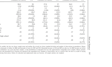
To facilitate comparability across the three datasets, we have restricted observations in the HRS, SEP, and CSS to individuals older than 50 and younger than 65 (for example, the highest age is 64). Table 1 presents a number of descriptive statistics for the three datasets. We observe that the Dutch samples exhibit a somewhat lower average and median age than the HRS. One should note that given the way the original HRS cohort has been drawn, average age in the HRS should increase over time, as no new younger individuals are added to the sample we are using if time progresses. Household size is somewhat higher in the HRS.
Income in the HRS is measured before tax, while in the Dutch data income is measured after tax, all in 1998 currencies. Although at first sight the different treat-ment of income in The Netherlands and in the United States may seem to cause problems, we believe that the way we use income in the quantitative analyses (by constructing quartiles of the distribution) is robust against the different treatment of taxes in both countries. For the use of quantiles it is only necessary that the ranking of incomes before and after tax is the same, which would appear a reasonable approx-imation in most cases.
Income in CSS is somewhat higher than in SEP. This is consistent with a suspicion of underestimation of income in SEP (comparison with external sources suggests an underestimation in SEP by about 10 percent on average). More strikingly, net worth and assets are much higher in CSS than in SEP. To a fairly large extent this can be ascribed to underestimation in SEP as well, as noted above. The CSS question-naire is much more detailed than the SEP questionquestion-naire, which makes it likely that more components of wealth are picked up than in the SEP. Furthermore, self-em-ployed are included in CSS, but not in the SEP. Alessie and Kapteyn (1999a) com-pare the SEP wealth data with external data published by Statistics Netherlands and find that average net worth in SEP may be underestimated by about 20 percent. Comparing this to sample means and medians reported for CSS in Table 1 would then suggest some overestimation in the CSS (even taking into account the omission of the self-employed from the SEP). This may point to a less than perfect reweighting of the data by means of the sample weights used in the CSS, resulting in an over-representation of high wealth households. Altogether, one may surmise that CSS and SEP provide respectively an upper and a lower bound on the wealth holdings of Dutch households.
Finally, with respect to Table 1, we should note that the definitions of education used in the two Dutch datasets differ, so that the distributions across education levels
Hurd
and
Kapteyn
397
Table 1
Descriptive Statistics for Three Datasets
HRS CSS SEP
Mean Median Mean Median Mean Median
(Standard Deviation) (N) (Standard Deviation) (N) (Standard Deviation) (N)
Age 58.0 58 57.0 57 56.9 57
(3.6) (41,998) (4.1) (6,464) (4.1) (6,175)
HH-size 2.7 2 2.2 2 2.0 2
(1.6) (29,020) (1.04) (3,659) (.89) (2,884)
Assets 302.2 126.7 161.6 125.3 103.3 85.3
(993.0) (29,020) (206.6) (3,099) (128.9) (2,884)
Liabilities 30.0 3.3 40.3 10.1 22.5 2.6
(75.6) (29,020) (68.1) (3,099) (40.2) (2,884)
Net worth 272.2 99.5 121.3 81.0 80.7 49.9
(991.1) (29,020) (175.6) (3,099) (108.4) (2,884)
HH income 56.7 38.6 25.8 22.2 24.2 21.5
(94.7) (29,020) (26.8) (3,753) (13.6) (2,791)
Education l.t. .22 0 .48 0 .47 0
High school (41,939) (6,444) (5,632)
High school .55 1 .22 0 .37 0
(41,939) (6,444) (5,632)
More than high school .23 0 .30 0 .16
(41,939) (6,444) (5,632)
Employed .62 1 .43 0 .40 0
(41,923) (5,454) (6,175)
Table 2
Distribution of Self-Assessed Health
HRS CSS SEP
Frequency % Frequency % Frequency % Excellent (HRS, CSS)/
very good (SEP) 7,845 18.8 841 19.7 858 13.8
Very good (HRS)/good
(CSS, SEP) 12,963 31.1 2,389 56.2 3,239 52.1
Good (HRS)/fair (CSS,
SEP) 11,876 28.5 820 19.3 1,814 29.2
Fair (HRS)/not so good
(CSS)/bad (SEP) 6,029 14.5 180 4.2 268 4.3
Poor (HRS, CSS)/very
bad (SEP) 2,926 7.0 23 0.5 38 0.6
Total 41,640 100 4,254 100 6,218 100
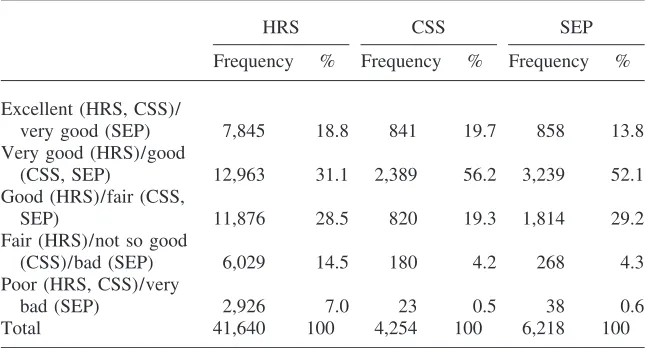
Frequencies are weighted; the definitions of the health categories vary by sample and are indicated in the category names in the table.
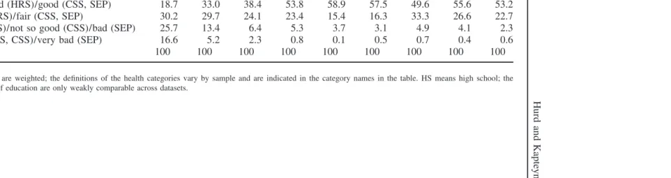
are not comparable. In the empirical analyses using education, we therefore always distinguish between the education definitions in CSS and SEP.
Table 2 provides the distribution of self-assessed health. The verbal labels associ-ated with the categories are given in the table as well. Clearly, the definitions of the health categories vary by dataset. The frequency distribution of health categories is more similar between the two Dutch datasets than between the HRS on the one hand and the Dutch datasets on the other hand. Taken at face value, the distribution of health levels is more dispersed in the American data. These differences may reflect true differences in health dispersion across the two countries or just be the effect of different wordings or different meanings attached to the verbal labels in different cultures (compare, for example, with Finch et al. 2002). These possibilities have to be kept in mind when analyzing the different patterns across socioeconomic groups in the two countries.
The relationship with education is qualitatively similar across the datasets (see Table 3) and shows the familiar pattern that the distribution of health shifts in the direction of better health if education goes up.
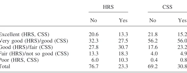
Tables 4, 5, and 6 show the relation between self-reported health and BMI, smok-ing, and alcohol consumption. These health behaviors are not available in SEP, so comparisons only involve HRS and CSS. Table 4 suggests that the Dutch weigh less than the Americans and confirm that a high BMI is bad for health (with minor nonmonotonicities in some places).
Hurd
and
Kapteyn
399
Table 3
Education and Self-Reported Health
HRS CSS SEP
⬍HS HS ⬎HS ⬍HS HS ⬎HS ⬍HS HS ⬎HS
Excellent (HRS, CSS)/very good (SEP) 8.7 18.7 28.9 16.6 21.8 22.6 11.4 13.3 21.1
Very good (HRS)/good (CSS, SEP) 18.7 33.0 38.4 53.8 58.9 57.5 49.6 55.6 53.2
Good (HRS)/fair (CSS, SEP) 30.2 29.7 24.1 23.4 15.4 16.3 33.3 26.6 22.7
Fair (HRS)/not so good (CSS)/bad (SEP) 25.7 13.4 6.4 5.3 3.7 3.1 4.9 4.1 2.3
Poor (HRS, CSS)/very bad (SEP) 16.6 5.2 2.3 0.8 0.1 0.5 0.7 0.4 0.6
Total 100 100 100 100 100 100 100 100 100
Table 4
BMI and Self-Reported Health
HRS CSS
Mean Median Mean Median
Excellent (HRS, CSS) 25.6 25.1 24.9 24.7
Very good (HRS)/good (CSS) 26.7 26.2 25.2 25.0
Good (HRS)/fair (CSS) 27.9 27.3 26.0 25.5
Fair (HRS)/not so good (CSS) 28.7 27.9 24.8 24.2
Poor (HRS, CSS) 28.4 27.4 29.7 26.0
Means and medians are weighted.
Table 5
Distribution of Self-Reported Health by Smoking or Nonsmoking
HRS CSS
No Yes No Yes
Excellent (HRS, CSS) 20.6 13.3 21.8 15.2
Very good (HRS)/good (CSS) 32.3 27.5 56.2 56.0
Good (HRS)/fair (CSS) 27.8 30.7 17.6 23.2
Fair (HRS)/not so good (CSS) 13.3 18.3 4.0 4.9
Poor (HRS, CSS) 6.0 10.3 0.4 0.8
Total 76.7 23.3 69.2 30.8
‘‘Yes’’ means the respondent smokes now; ‘‘No’’ means the respondent does not smoke now. The bottom row gives the percentages of smokers and nonsmokers in both samples. All percentages are based on weighted data.
that drinking more than four glasses of alcohol is bad for health in the United States and good for health in The Netherlands.
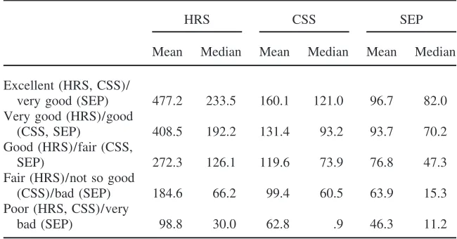
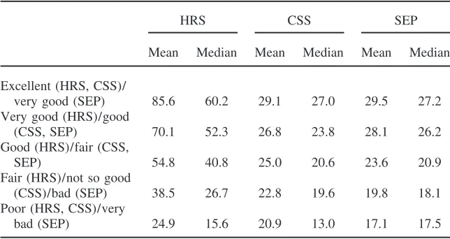
There is a monotonic relationship between health and wealth in both countries (Table 7). The same is true of the relation between health and income (Table 8), but the relation is less steep in The Netherlands than in the United States. In part, this simply reflects the more equal income distribution in The Netherlands.
Hurd and Kapteyn 401
Table 6
Distribution of Self-Reported Health by Alcohol Consumption
HRS CSS
No Yes No Yes
Excellent (HRS, CSS) 16.8 11.2 19.5 21.7
Very good (HRS)/good (CSS) 32.1 24.8 56.1 56.5
Good (HRS)/fair (CSS) 28.9 36.0 19.5 17.6
Fair (HRS)/not so good (CSS) 15.2 20.4 4.3 4.0
Poor (HRS, CSS) 6.9 7.5 0.6 0.3
Total 97.8 2.2 89.6 10.4
‘‘Yes’’ means the respondent drinks more than four glasses of alcohol per day; ‘‘No’’ means the respondent drinks less or not at all. The bottom row gives the percentages of both groups in both samples. All percent-ages are based on weighted data.
Table 7
Health and Wealth
HRS CSS SEP
Mean Median Mean Median Mean Median Excellent (HRS, CSS)/
very good (SEP) 477.2 233.5 160.1 121.0 96.7 82.0 Very good (HRS)/good
(CSS, SEP) 408.5 192.2 131.4 93.2 93.7 70.2
Good (HRS)/fair (CSS,
SEP) 272.3 126.1 119.6 73.9 76.8 47.3
Fair (HRS)/not so good
(CSS)/bad (SEP) 184.6 66.2 99.4 60.5 63.9 15.3
Poor (HRS, CSS)/very
bad (SEP) 98.8 30.0 62.8 .9 46.3 11.2
Money amounts are in thousands of dollars for HRS and thousands of euros for SEP and CSS. Wealth is household net worth.
or third quartile, and high is the highest quartile. We code income and wealth by quartiles separately for each year and for each dataset.4The purpose of the tables is not to suggest any causality, but rather to characterize the strength of the relationship between health and SES in both countries. In the table, we show results for The
Table 8
Health and Income
HRS CSS SEP
Mean Median Mean Median Mean Median Excellent (HRS, CSS)/
very good (SEP) 85.6 60.2 29.1 27.0 29.5 27.2
Very good (HRS)/good
(CSS, SEP) 70.1 52.3 26.8 23.8 28.1 26.2
Good (HRS)/fair (CSS,
SEP) 54.8 40.8 25.0 20.6 23.6 20.9
Fair (HRS)/not so good
(CSS)/bad (SEP) 38.5 26.7 22.8 19.6 19.8 18.1
Poor (HRS, CSS)/very
bad (SEP) 24.9 15.6 20.9 13.0 17.1 17.5
Money amounts are in thousands of dollars for HRS and thousands of euros for SEP and CSS. Household incomes in CSS and SEP are after tax; for HRS incomes are before tax.
Netherlands based on pooled data of CSS and SEP. When pooling CSS and SEP we retain different education dummies for the two datasets in light of the differences in definition, as discussed earlier. A test of equality of the income/wealth dummies across the two datasets does not lead to rejection (χ2(8) 9.37 p
⫽0.31), which justifies the pooling. Table 9 shows a much steeper gradient of health with SES for HRS than for CSS/SEP (for instance the odds ratio of income high and wealth high is 8.61 for HRS and 2.46 for CSS/SEP), although the relation is statistically highly significant in all datasets. Education also has a highly significant relation with health, but again in The Netherlands the relation is less steep.
IV. The Impact of Health on Wealth and Income
Changes
We have established that both the U.S. data and the Dutch data show a strong positive cross-section association between health and indicators of socioeco-nomic status. In keeping with the theoretical model, we now consider the effect of health status on income and wealth changes. The relation between health status and income changes is similar to that in Equation 4 above.
Hurd and Kapteyn 403
Table 9
The Cross-Section Association between Health and SES in the Two Countries
Odds Odds
HRS Ratios CSS/SEP Ratios
Income low, wealth medium 0.797 2.22 0.098 1.10
(14.55)** (0.80)
Income low, wealth high 1.681 5.37 0.059 1.06
(18.55)** (0.33)
Income medium, wealth low 0.971 2.64 0.277 1.32
(18.36)** (2.40)*
Income medium, wealth medium 1.389 4.01 0.603 1.83
(28.38)** (5.74)**
Income medium, wealth high 1.814 6.13 0.615 1.85
(30.99)** (4.96)**
Income high, wealth low 1.406 4.08 0.451 1.57
(12.71)** (1.86)
Income high, wealth medium 1.829 6.22 0.742 2.10
(30.97)** (6.07)**
Income high, wealth high 2.153 8.61 0.902 2.46
(36.61)** (7.18)**
High school 0.681 1.98
(17.85)**
More than high school 1.058 2.88
(21.98)**
High school (SEP) 0.051 1.05
(0.61)
More than high school (SEP) 0.375 1.45
(3.06)**
High school (CSS) 0.315 1.37
(2.52)*
More than high school (CSS) 0.168 1.18
(1.42)
Observations 42,193 9,423
Pseudo-R2 0.07 0.03
Chi squared income/wealth 1,520.32 84.38
p-value 0.00 0.00
Robustz-statistics in parentheses.
*⫽significant at 5 percent; **⫽significant at 1 percent.
The
Journal
of
Human
Resources
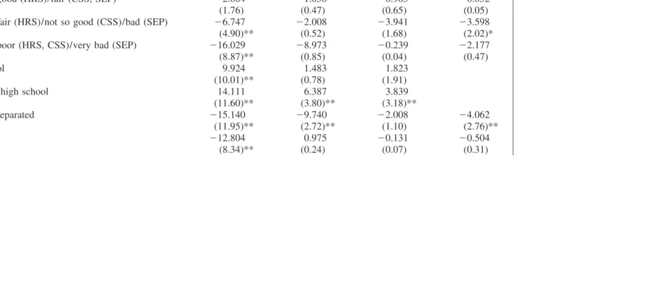
Table 10
Health Levels and Wealth Changes
(1) (2) (3) (4)
HRS CSS SEP CSS/SEP
Health⫽very good (HRS)/ good (CSS, SEP) 0.380 3.125 1.577 1.901
(0.34) (1.74) (1.25) (2.12)*
Health⫽good (HRS)/fair (CSS, SEP) ⫺2.004 ⫺1.058 0.905 ⫺0.052
(1.76) (0.47) (0.65) (0.05)
Health⫽fair (HRS)/not so good (CSS)/bad (SEP) ⫺6.747 ⫺2.008 ⫺3.941 ⫺3.598
(4.90)** (0.52) (1.68) (2.02)*
Health⫽poor (HRS, CSS)/very bad (SEP) ⫺16.029 ⫺8.973 ⫺0.239 ⫺2.177
(8.87)** (0.85) (0.04) (0.47)
High school 9.924 1.483 1.823
(10.01)** (0.78) (1.91)
More than high school 14.111 6.387 3.839
(11.60)** (3.80)** (3.18)**
Divorced/separated ⫺15.140 ⫺9.740 ⫺2.008 ⫺4.062
(11.95)** (2.72)** (1.10) (2.76)**
Widowed ⫺12.804 0.975 ⫺0.131 ⫺0.504
Hurd
and
Kapteyn
405
Not married ⫺9.500 ⫺5.380 1.144 ⫺0.182
(5.37)** (1.71) (0.95) (0.18)
High school (SEP) 1.662
(1.94)
More than high school (SEP) 2.916
(2.59)**
High school (CSS) 3.404
(2.82)**
More than high school (CSS) 7.922
(7.83)**
Observations 30,625 2,509 3,918 6,518
F-test health 27.76 2.00 1.92 4.19
p-value 0.00 0.09 0.00 0.00
F-test education 73.90 7.72 5.34 15.85
p-value 0.00 0.00 0.10 0.00
Absolute value of t-statistics in parentheses.
*⫽significant at 5 percent; **⫽significant at 1 percent.
category lags by 3.6 percent. For the separate Dutch data, we find some weak effects, but these are only statistically significant in the SEP. Also, note that a test for equality of health effects on wealth in the two Dutch datasets leads to rejection at the 2 percent level. Thus, the pooled results are in principle based on a misspecified model. Hence, we report both results based on the separate datasets and results based on the pooled data.
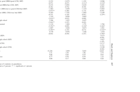
The effects of health on income are statistically marginally significant in the HRS and significant in the pooled SEP/CSS data (Table 11). A test for equality of the health effects in CSS and SEP leads to acceptance (p ⫽ 0.55). This outcome is somewhat surprising in view of the relatively extensive income maintenance pro-grams in The Netherlands. The significance of the effects in The Netherlands seems to be largely driven by the relatively large effect for poor/very bad health. For the other health categories, the effects are about equal to those for the U.S. data, if not smaller.
V. The Impact of Wealth and Income on Health
Transitions
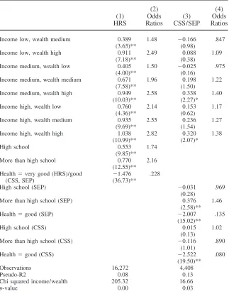
We quantify the effects of wealth and income on health changes via ordered logit estimation of the rate of health transition from one wave to another. We consider transitions from three initial health levels: from health being in the top two categories, from health being in the middle category, and from health being in the two bottom categories. Tables 12 through 14 present the results. As in Section III, we also consider estimation results for pooling the CSS and SEP data (while keeping separate education dummies). Since in all three cases we accept the null hypothesis that income and wealth effects are the same across SEP and CSS, we only present the pooled results for the Dutch data.
Table 12 gives the estimated effects on the transition from excellent/very good health in HRS, or from excellent or good health (CSS), or from very good or good (SEP) to each of the possible five destination states. A positive coefficient increases the chances of maintaining health in the top category; any transition will be to the middle category rather than to the bottom categories. We have added a dummy for health being very good (HRS) or good (CSS, SEP) to indicate where in the top categories one is at baseline.
Income and wealth have a significant influence on health transitions in both coun-tries, but the effect appears to be considerably larger in the United States than in The Netherlands. This would suggest (compare with Equation 4) thatγis bigger in the United States than in The Netherlands. In both countries it also appears that wealth is more important than income. In The Netherlands the combined effect of income and wealth is dominated by wealth. In the United States we observe a nonlin-earity in the effect of income and wealth: An increase in wealth at all income levels increases the odds of remaining in the top health category; an increase in income only increases the odds when wealth is low or medium, not when wealth is high.
transi-Hurd
and
Kapteyn
407
Table 11
Health Levels and Income Changes
(1) (2) (3) (4)
HRS CSS SEP CSS/SEP
Health⫽very good (HRS)/good (CSS, SEP) ⫺0.331 ⫺0.273 ⫺1.221 ⫺0.946
(0.57) (0.27) (2.11)* (2.19)*
Health⫽good (HRS)/fair (CSS, SEP) ⫺0.151 ⫺0.991 ⫺0.245 ⫺0.201
(0.26) (0.76) (0.38) (0.40)
Health⫽fair (HRS)/not so good (CSS)/bad (SEP) ⫺1.882 4.059 ⫺1.224 ⫺0.503
(2.67)** (1.80) (1.14) (0.58)
Health⫽poor (HRS, CSS)/very bad (SEP) ⫺0.303 ⫺7.701 ⫺2.082 ⫺5.189
(0.33) (1.20) (0.81) (2.29*)
High school 1.319 0.026 0.002
(2.63)** (0.02) (0.00)
More than high school 2.266 1.022 0.457
(3.64)** (1.07) (0.82)
Divorced/separated ⫺2.134 1.804 1.751 1.766
(3.35)** (0.89) (2.10)* (2.48)*
Widowed ⫺2.607 3.026 0.673 2.561
(3.39)** (1.35) (0.73) (3.23)**
Not married 0.739 0.876 1.046 1.010
(0.84) (0.49) (1.87) (1.98)*
High school (SEP) 0.215
(0.50)
More than high school (SEP) 0.827
(1.45)
High school (CSS) ⫺0.717
(1.31)
More than high school (CSS) ⫺0.188
(0.40)
Observations 31,226 2,895 3,643 6,624
F-test health 2.31 1.59 1.96 2.75
p-value 0.06 0.50 0.10 0.03
F-test education 6.77 0.70 0.39 1.32
p-value 0.00 0.17 0.68 0.26
Absolute value of t-statistics in parentheses.
Ordered Logits: Health in the Top Two Categories at Baseline
(2) (4)
(1) Odds (3) Odds
HRS Ratios CSS/SEP Ratios Income low, wealth medium 0.389 1.48 ⫺0.166 .847
(3.65)** (0.98)
Income low, wealth high 0.911 2.49 0.088 1.09 (7.18)** (0.38)
Income medium, wealth low 0.405 1.50 ⫺0.025 .975 (4.00)** (0.16)
Income medium, wealth medium 0.671 1.96 0.198 1.22 (7.58)** (1.50)
Income medium, wealth high 0.949 2.58 0.338 1.40 (10.03)** (2.27)*
Income high, wealth low 0.760 2.14 0.153 1.17 (4.36)** (0.62)
Income high, wealth medium 0.935 2.55 0.236 1.27 (9.69)** (1.54)
Income high, wealth high 1.038 2.82 0.320 1.38 (10.99)** (2.07)*
High school 0.553 1.74 (9.85)** More than high school 0.770 2.16
(12.55)** Health⫽very good (HRS)/good ⫺1.476 .228
(CSS, SEP) (36.73)**
High school (SEP) ⫺0.031 .969 (0.28)
More than high school (SEP) 0.376 1.46 (2.58)** Health⫽good (SEP) ⫺2.007 .135
(15.02)** High school (CSS) 0.015 1.02
(0.13)
More than high school (CSS) ⫺0.116 .890 (1.01)
Health⫽good (CSS) ⫺2.522 .080 (19.50)** Observations 16,272 4,408 Pseudo-R2 0.08 0.13 Chi squared income/wealth 205.32 16.66
p-value 0.00 0.03
Robustz-statistics in parentheses.
*⫽significant at 5 percent; **⫽significant at 1 percent.
Hurd and Kapteyn 409
Table 13
Ordered Logits: Health in the Middle Category at Baseline
(2) (4)
(1) Odds (3) Odds
HRS Ratios CSS/SEP Ratios
Income low, wealth medium 0.327 1.39 0.154 1.17
(3.52)** (0.79)
Income low, wealth high 0.573 1.77 ⫺0.143 .867
(3.44)** (0.51)
Income medium, wealth low 0.407 1.50 0.181 1.20
(4.46)** (0.84)
Income medium, wealth medium 0.587 1.80 0.327 1.39
(7.20)** (1.87)
Income medium, wealth high 0.785 2.19 0.179 1.20
(7.79)** (0.82)
Income high, wealth low 0.640 1.90 ⫺0.699 .497
(3.73)** (1.28)
Income high, wealth medium 0.720 2.05 0.537 1.71
(7.36)** (2.22)*
Income high, wealth high 0.769 2.16 0.818 2.27
(7.90)** (3.36)*
High school 0.277 1.32
(5.44)**
More than high school 0.459 1.58
(6.93)**
High school (SEP) 0.021 1.20
(0.14)
More than high school (SEP) 0.367 1.44
(1.70)
High school (CSS) 0.440 1.55
(1.50)
More than high school (CSS) 0.406 1.50
(1.74)
Observations 9,857 1,568
Pseudo-R2 0.02 0.02
Chi squared income/wealth 88.09 20.24
p-value 0.00 0.01
Robustz-statistics in parentheses.
*⫽significant at 5 percent; **⫽significant at 1 percent.
Ordered Logits: Health in the Bottom Two Categories at Baseline
(2) (4)
(1) Odds (3) Odds
HRS Ratios CSS/SEP Ratios Income low, wealth medium 0.214 1.24 ⫺0.243 .784
(2.94)** (0.51)
Income low, wealth high 0.161 1.17 0.456 1.56 (0.85) (0.74)
Income medium, wealth low 0.332 1.39 ⫺0.195 .823 (4.29)** (0.33)
Income medium, wealth medium 0.436 1.55 0.271 1.31 (6.27)** (0.57)
Income medium, wealth high 0.619 1.86 ⫺0.554 .575 (5.98)** (0.80)
Income high, wealth low 0.520 1.68 ⫺0.986 .373 (2.14)** (1.06)
Income high, wealth medium 0.803 2.32 0.389 1.48 (6.57)** (0.59)
Income high, wealth high 0.913 2.50 0.621 1.86 (7.31)** (0.72)
High school 0.174 1.19 (3.53)**
More than high school 0.256 1.29 (2.81)**
Health⫽fair (HRS)/not so good 1.803 6.06 (CSS)/bad (SEP) (29.78)**
High school (SEP) ⫺0.230 .795 (0.64)
More than high school (SEP) ⫺0.405 .667 (0.55)
Health⫽bad (SEP) 1.704 5.50 (2.20)*
High school (CSS) ⫺0.442 .642 (0.85)
More than high school (CSS) 0.186 1.20 (0.31)
Health⫽not so good (CSS) 3.181 24.1 (4.35)** Observations 7,799 296 Pseudo-R2 0.09 0.11 Chi squared income/wealth 87.45 7.73
p-value 0.00 0.46
Robustz-statistics in parentheses.
*⫽Significant at 5 percent; **⫽significant at 1 percent.
Hurd and Kapteyn 411
tion to better health or reduces the probability of a transition to worse health. The wealth income interactions are statistically significant in both countries. As before, the economic variables appear to have a stronger effect in the HRS than in the Dutch data, but the differences are fairly minor.
In Table 14, the baseline category is fair or poor for HRS, not so good or poor for CSS, and bad or very bad for SEP. The effects of income and wealth on the health transitions are now totally insignificant in the Dutch data, possibly due to the modest number of observations.
VI. Interpretation and Conclusions
The conceptual model presented in Section II refers to the relation-ship between health and income. The theoretical relationrelation-ship between wealth and health is considerably more complicated involving the propensity to consume out of income and the interest rate. We have not fully developed that theory beyond the observation that in populations where there is large variation in wealth there should be large variation in health. Therefore, when discussing the results in relation to the model we concentrate on the results relating income and health. We should reiterate however the observation in Section I that healthier individuals have more reasons to save for retirement, but that this reason is substantially less prominent in The Netherlands, where most retirement consumption is financed out of annuity income. We do indeed find that the effect of health on wealth is considerably smaller in the United States than in The Netherlands.
Based on the cross-section estimations of the effects of income and wealth on health status (Table 9), we can calculate the average change in relative risk holding constant wealth by averaging the relative risk over each wealth category. For exam-ple, in the HRS the average risk of being in a higher health category for someone in the top income quartile is computed to be 2.49 greater than the risk of someone in the lowest income quartile. In The Netherlands the relative risk is 1.90. Relating this result back to our conceptual model (compare with Equations 11 and 16), it indicates that γ/αis somewhat greater in the United States. That is, the change in health is more strongly related to the income level in the United States than in The Netherlands.
Based on the three panel estimations (Tables 12, 13, and 14) we may calculate an estimate ofγin a similar way by assuming that these equations are the empirical counterpart of Equation 4. The estimations not only hold wealth constant, but also holds baseline health constant in one of the three health status categories. In the HRS among those in the top income quartile the average relative risk of transiting to a higher health state can be calculated as 1.66 greater than the risk of someone in the lowest income quartile. In The Netherlands, the risk is 1.23 greater. Thus, the panel transitions indicate a higher level of γin the United States than in The Netherlands.
The
Journal
of
Human
Resources
Table 11
Health Levels and Income Changes
(1) (2) (3) (4)
HRS CSS SEP CSS/SEP
Health⫽very good (HRS)/good (CSS, SEP) ⫺0.331 ⫺0.273 ⫺1.221 ⫺0.946
(0.57) (0.27) (2.11)* (2.19)*
Health⫽good (HRS)/fair (CSS, SEP) ⫺0.151 ⫺0.991 ⫺0.245 ⫺0.201
(0.26) (0.76) (0.38) (0.40)
Health⫽fair (HRS)/not so good (CSS)/bad (SEP) ⫺1.882 4.059 ⫺1.224 ⫺0.503
(2.67)** (1.80) (1.14) (0.58)
Health⫽poor (HRS, CSS)/very bad (SEP) ⫺0.303 ⫺7.701 ⫺2.082 ⫺5.189
(0.33) (1.20) (0.81) (2.29*)
High school 1.319 0.026 0.002
(2.63)** (0.02) (0.00)
More than high school 2.266 1.022 0.457
(3.64)** (1.07) (0.82)
Divorced/separated ⫺2.134 1.804 1.751 1.766
(3.35)** (0.89) (2.10)* (2.48)*
Widowed ⫺2.607 3.026 0.673 2.561
(3.39)** (1.35) (0.73) (3.23)**
Not married 0.739 0.876 1.046 1.010
(0.84) (0.49) (1.87) (1.98)*
High school (SEP) 0.215
(0.50)
More than high school (SEP) 0.827
(1.45)
High school (CSS) ⫺0.717
(1.31)
More than high school (CSS) ⫺0.188
(0.40)
Observations 31,226 2,895 3,643 6,624
F-test health 2.31 1.59 1.96 2.75
p-value 0.06 0.50 0.10 0.03
F-test education 6.77 0.70 0.39 1.32
p-value 0.00 0.17 0.68 0.26
Absolute value of t-statistics in parentheses.
Hurd and Kapteyn 413
nature of the health measure and the definitional differences between the categories in the two countries a comparison is somewhat tenuous, but qualitatively it appears that α, as derived from Table 11, is greater in The Netherlands than in the United States, at least as measured by the largest of the coefficients (on poor health). Thus, we find broadly consistent estimates of the underlying parameters of our theoretical model. However, we clearly need better measures that can be compared with more confidence across the countries. The current datasets do not provide such comparable measures. Also, we note that these calculations ignore possible differences in the variance of unobserved heterogeneity in both countries (λin Equation 19).
We began the cross-country comparison with the observation that if national poli-cies alter both the financing of health care services and other inputs into health pro-duction, and the relationship between health and income, we should find predictable differences in the relationship between health and income in cross-section and in panel. In The Netherlands, health care is universal and practically independent of income whereas that would not be the case in the United States. In The Netherlands, income redistribution programs reduce the strength of the relationship between health and income. We found differing relationships between health and income in the two countries, and the differences are consistent with what our conceptual model would predict.
Clearly, our analysis invites several improvements. On the conceptual side, a more complex model relating health, wealth, and income in a three-equation system of differential equations appears to be a natural extension. On the data side, one would want to consider more countries and a much wider array of health measures. Al-though at this moment micropanel datasets measuring health, income, and wealth are only available in a very limited set of countries, the movement in various countries to emulate the U.S. Health and Retirement Study provides an exciting perspective on making progress in quantifying the relation of health and SES and the role of institu-tions in amending this relainstitu-tionship.
References
Adams, Peter, Michael D. Hurd, Daniel McFadden, Angela Merrill, and Tiago Ribeiro. 2003. ‘‘Healthy, Wealthy, and Wise? Tests for Direct Causal Paths between Health and Socioeconomic Status.’’Journal of Econometrics112:3–56.
Alessie, Robert, Annamaria Lusardi, and Trea Aldershof. 1997. ‘‘Income and Wealth over the Life Cycle: Evidence from Panel Data.’’The Review of Income and Wealth43:1–32. Alessie, Robert, and Arie Kapteyn. 1999a. ‘‘Savings, Pensions and Portfolio Choice in The
Netherlands.’’ Amsterdam: Free University.
Alessie, Robert, Annamaria Lusardi, and Arie Kapteyn. 1999b. ‘‘Savings after Retirement: Evidence from Three Different Surveys.’’Labour Economics6:277–310.
Avery, Robert B., Gregory E. Elliehausen, and Arthur B. Kennickell. 1988. ‘‘Measuring Wealth with Survey Data: An Evaluation of the 1983 Survey of Consumer Finances.’’
The Review of Income and Wealth34:339–69.
Avery, Robert, and Arthur Kennickell. 1991. ‘‘Household Saving in the U.S.’’Review of Income and Wealth37:409–32.
Boffetta, Paolo, and Lawrence Garfinkel. 1990. ‘‘Alcohol Drinking and Mortality among Men Enrolled in an American Cancer Society Prospective Study.’’Epidemiology1(5): 343–48.
Camphuis, Herman. 1993. ‘‘Checking, Editing and Imputation of Wealth Data of the Netherlands Socio-Economic Panel for the period 87–89.’’ VSB Progress Report n. 10, CentER. The Netherlands: Tilburg University.
Davies, James. 1979. ‘‘On the Size Distribution of Wealth in Canada.’’Review of Income and Wealth25:237–59.
Feinstein, Jonathan. 1993. ‘‘The Relationship between Socioeconomic Status and Health: A Review of the Literature.’’Milbank Quarterly71(2):279–322.
Finch, Brian K., Robert A. Hummer, Maureen Reindl, William A. Vega. 2002. ‘‘The Valid-ity of Self-Rated Health among Latino(a)s.’’ Berkeley: UniversValid-ity of California, School of Public Health. Mimeo.
Fuchs, Victor R. 1982. ‘‘Time Preference and Health: an Explanatory Study. InEconomic Aspects of Health. Chicago: University of Chicago Press.
Goldman, Noreen. 2001. ‘‘Social Inequalities in Health: Disentangling the Underlying Mechanisms.’’ InPopulation Health and Aging—Strengthening the Dialogue Between Epidemiology and Demography, ed. Maxine Weinstein, Albert I. Hermalin, and Michael A. Stoto.Annals of the New York Academy of Sciences954:118–39.
Grossman, Michael. 1972.The Demand for Health-A Theoretical and Empirical Investiga-tion. New York: National Bureau of Economic Research.
Hill, Daniel H., and Nancy A. Mathiowetz. 1998. ‘‘The Empirical Validity of the HRS Medical Expenditure Data: A Model to Account for Different Reference Periods.’’ Ann Arbor: HRS Working Paper Series.
Hurd, Michael D. 1987. ‘‘Saving of the Elderly and Desired Bequests.’’American Eco-nomic Review77:289–312.
———. 1989. ‘‘Mortality Risks and Bequests.’’Econometrica57:779–813.
———. 1998. ‘‘Mortality Risks and Consumption by Couples.’’ Santa Monica: RAND Working Paper DRU-2061.
Hurd, Michael D., and Kathleen McGarry. 1995. ‘‘Evaluation of the Subjective Probabili-ties of Survival in the HRS.’’Journal of Human Resources30:S268–S292.
Hurst, Erik, Ming Ching Luoh, and Frank P. Stafford. 1998. ‘‘Wealth Dynamics of Ameri-can Families: 1984–1994.’’Brooking Papers on Economic Activity1:267–337.
Juster, F. Thomas, and Richard M. Suzman. 1995. ‘‘An Overview of the Health and Retire-ment Study.’’Journal of Human Resources30:S7–S56.
Kitagawa, Evelyn M., and Philip M. Hauser. 1973.Differential Mortality in the United States: A Study in Socioeconomic Epidemiology. Cambridge, Mass.: Harvard University Press.
Marmot, Michael G., George Davey Smith, Stephen Stansfeld, Chandra Patel, Fiona North, J. Head, Ian White, Eric Brunner, and Amanda Feeny. 1991. ‘‘Health Inequalities among British Civil Servants: The Whitehall II Study.’’Lancet, June 8, pp. 1387– 93.
McClellan, Mark. 1998. ‘‘Health Events, Health Insurance and Labor Supply: Evidence from the Health and Retirement Survey.’’ InFrontiers in the Economics of Aging, ed. David Wise, 301–46. Chicago: University of Chicago Press.
Robert, Stephanie, and James House. 1994. ‘‘Socioeconomic Status and Health Over the Life Course.’’ InSocial Structures, Quality of Life, and Aging, ed. Ronald P. Abeles, Helen C. Gift, and Marcia G. Ory, 253–74. New York: Springer Publishing Company. ———. 2000. ‘‘Socioeconomic Inequalities in Health: Integrating Individual-,
Hurd and Kapteyn 415
Shaper, A. G. 1990. ‘‘Alcohol and Mortality: A Review of Prospective Studies.’’British Journal of Addiction85:837–47.
Smith, James P. 1999. ‘‘Healthy Bodies and Thick Wallets: The Dual Relationship be-tween Health and Economic Status.’’Journal of Economic Perspectives13:145–66. Van Doorslaer, Eddy, Adam Wagstaff, Han Bleichrodt, Samuel Calonge, Ulf-G. G.
Gerd-tham, Michael Gerfin, Jose´ Geurts, Lorna Gross, Unto Ha¨kkinen, Robert E. Leu, Owen O’Donnell, Carol Propper, Frank Puffer, Marisol Rodriguez, Gun Sundberg, Olaf Winkel-hake. 1997. ‘‘Income-Related Inequalities in Health: Some International Comparisons.’’
Journal of Health Economics16:93–112.