Participation in Sweden
Lennart Flood
Jörgen Hansen
Roger Wahlberg
A B S T R A C T
We formulate and estimate a structural, static model of household labor sup-ply and multiple welfare program participation. Given the complicated nature of both the income tax schedule and the benefit rules for different welfare programs, we use a detailed micro simulation model to generate accurate budget sets for each work-welfare combination. We also use high-quality data on earnings and other types of incomes obtained both from employers and from income tax records. The results suggest that labor sup-ply among two-parent families in Sweden is quite inelastic. A policy simula-tion designed to increase labor supply incentives for low income families generated substantial positive welfare effects, despite only minor changes in labor supply and in welfare participation.
I. Introduction
An extensive literature in economics discusses the impact of income taxes and government transfer programs on labor supply behavior (see, for instance, the survey in Blundell and MaCurdy 1999). Most of the existing work regarding the
Lennart Flood is a professor of economics at Göteborg University and affiliated with IZA. Jörgen Hansen is an assistant professor of economics at Concordia University, Canada, and affiliated with CEPR, CIRANO, CIREQ, and IZA. Roger Wahlberg is an assistant professor of economics at Göteborg University, Sweden. The authors would like to thank two anonymous referees, Rob Euwals, Magnus Lofstrom, Thomas MaCurdy, and Arthur van Soest, as well as seminar participants at Concordia University, Göteborg University, IUPU Indianapolis, IZA, and Uppsala University for helpful comments and suggestions. Financial support from the Swedish Counsel for Social Research and from the Jan Wallander and Tom Hedelius Foundation for Research in Economics is gratefully acknowledged. Data for this paper are available from Statistics Sweden. Contact the authors for information about how to apply for access to the data. Lennart Flood, Box 640, SE 405 30 Göteborg, Sweden. Email: <Lennart.Flood@economics.gu.se>.
[Submitted February 2001; accepted June 2003]
ISSN 022-166XE-ISSN 1548-8004 © 2004 by the Board of Regents of the University of Wisconsin System
disincentive effects of transfer programs has focused on the labor supply responses of single women to changes in the Aid to Families with Dependent Children (AFDC) program (Levy 1979; Moffitt 1986).1Recently, this literature was extended to study the impact of the combination of cash benefits and in-kind benefits on single women’s labor supply (Moffitt 1992; Keane and Moffitt 1998) and on householdlabor supply (Hagstrom 1996; Hoynes 1996).
Although the effects of government transfer programs on labor supply behavior in the United States is relatively well known, much less is known about such effects in other, less market-oriented countries, such as Sweden. Similar to the United States, Sweden also substantially changed the structure of its public cash assistance programs to low-income families in the 1990s.2However, instead of removing national eligibil-ity and payment rules, as was done in the United States when AFDC was replaced with TANF in 1996, Sweden decided to remove any local variations in eligibility and payment rules.3Until 1998, the benefit levels of social assistance (SA)—one of the major means-tested cash assistance programs to low-income households in Sweden— were determined in each of the 288 municipalities in Sweden. However, as of January 1, 1998, the regional variations in the benefit levels were replaced by a national, uniform benefit level.4 Although most SA recipients are female-headed households, benefits are available to eligible two-parent households. Despite recent interest about the program’s effect on labor supply and welfare use, there exists little empirical evidence of these effects on the behavior of single mothers (recent exemp-tions are Andren 2003 and Flood, Pylkkanen, and Wahlberg 2003) and, as far as we know, no evidence on the behavior of two-parent households.
In this paper, we estimate the effects of income taxes and government transfer pro-grams on the labor supply behavior of two-parent families in Sweden. We formulate and estimate a structural, static model of household labor supply and multiple welfare program participation—SA and housing allowance (HA)—in which hours of work for both spouses as well as welfare participation is chosen to maximize household utility subject to a budget constraint. There are at least two problems to consider when for-mulating and estimating such a model. First, the model must deal appropriately with the complicated nature of both the income tax schedule and the benefit rules for dif-ferent transfer programs. Both income taxes and means-tested benefits combine to generate highly nonlinear and sometimes nonconvex budget constraints. Second, because benefit entitlement is determined by householdincome, which implies that the labor market decision of one household member can influence the budget con-straint for the other member, a traditional labor supply model, such as the one pro-posed by Hausman (1985) or MaCurdy, Green, and Paarsch (1990), is computationally infeasible. Instead, the model must have the capacity of dealing with decisions at the household level as opposed to the individual level.
To address the first problem mentioned above, we combine administrative data with detailed information on income and earnings from different sources. These data are
1. In August 1996, AFDC—the primary cash assistance program for low-income families—was replaced with the Temporary Assistance for Needy Families (TANF) block grant.
obtained both from income-tax registers as well as from employers. It is especially important in a study such as this to have access to high-quality data, partly because there tend to be serious under-reporting of welfare participation in traditional survey data, but also because it allows us to obtain very precise budget constraints for differ-ent hours of work combinations. Moreover, by using employer provided wages as opposed to self-reported wages, we reduce the potential problems with “division-bias” and measurement errors in wages. To our knowledge, this paper is the first to use high-quality data in a structural household labor supply model. Further, in addi-tion to using high-quality data, we use a micro-simulaaddi-tion model—developed and used by Statistics Sweden and the Swedish Ministry of Finance—to generate budget sets for each household and for each hours and welfare participation combination. The simulation model incorporates many details of the existing tax and government transfer systems and also provides details on childcare costs and other fixed costs of work. Given the complicated nature of both the income tax schedule and the benefit rules for different transfer programs, it is virtually impossible to obtain accurate budget constraints using simple approximations. Finally, we pool data from 1993 and 1999, in part because they represent times of recession (1993) and economic growth (1999), but also because they provide us with information before and after the reform in the benefit levels for SA.
To deal with the second problem mentioned above, we decided to build on a joint labor supply model with discrete hours of work, following van Soest (1995); Hoynes (1996); Keane and Moffitt (1998), and Blundell et al. (2000). The discrete approach to labor supply estimation has a number of advantages over continuous methods. Firstly, it is straightforward to deal with nonlinear income taxes in a manner that does not impose the Slutsky restriction on the parameters of the model. Secondly, the pref-erence model is fully structural and economic theory is testable. Thirdly, it is feasible to incorporate preference heterogeneity in the model. Finally, it is straightforward to include as many details as possible regarding the budget set. Following Moffitt (1983) and Hoynes (1996), we extend the basic discrete labor supply model by adding terms for the possibility of stigma effects associated with participation in different welfare programs. Moreover, in order to reduce the potential problem associated with map-ping a continuum of hours into a finite set of classes, we add the possibility of classi-fication errors as in MaCurdy, Green, and Paarsch (1990) and Hoynes (1996). Finally, we allow for preference heterogeneity using a semiparametric approach building on Heckman and Singer (1984).
The results suggest that labor supply among two-parent families in Sweden is quite inelastic. For instance, a 10 percent wage increase for husbands is associated with an average increase in hours of work of 0.5 percent. For women, the corresponding labor supply response is an increase by 1 percent. Although a small wage elasticity for men is not uncommon in the literature, our result for women is generally lower than most of the existing results. Regarding the effects on participation in SA and in the HA pro-gram, we find that increases in the maximum benefit levels are associated with mod-erate increases in participation rates. Specifically, an increase in the maximum benefit level for SA (HA) with 25 percent yields an increase in the participation rate of 4.2 percent (3.1 percent).
SA and HA. In Sweden, as well as in many other countries, there is a concern about the high implicit marginal tax rates of an increase in working hours for low-income earners. These effects are due to a combination of a relatively high income tax rate on low earnings combined with a 100 percent implicit tax on welfare benefits. The results from the policy simulation indicate that a significant reduction in income taxes for low-income earners along with a 25 percent reduction in the maximum benefit levels in both SA and HA generate substantial welfare effects. Using equivalent variation (EV) as our measure of the welfare effect associated with the tax and welfare change, we find that there are welfare gains for virtually everyone in the sample from the tax and transfer change. However, there are dramatic differences in EV depending on the level of prereform household income. The estimated average EV for the poorest 10 percent is SEK 11,345 per year compared with SEK 57,195 per year for the richest 10 percent.
The remainder of this paper is organized as follows. Section II provides a descrip-tion of SA and HA in Sweden. In Secdescrip-tion III, the main features of the Swedish income tax system is presented. Section IV presents the economic model and the empirical specification while Section V describes the data used in the analysis. In Section VI we present the results, while Section VII concludes the paper.
II. SA and HA in Sweden
The Swedish welfare system is well known internationally for the high degree of income security that it provides for its residents. Recently, this gener-ous system has been the target of a number of reforms, mainly due to the recession that hit Sweden in the early 1990s.
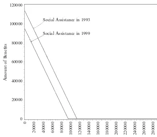
As an ultimate safety net, people in Sweden are covered by SA. In order to be eli-gible for SA, all other welfare programs, such as unemployment compensation, HA, child allowance and various pensions must be exhausted first. The benefit levels vary across family types and are intended to cover expenses essential for a “decent” living. To be eligible for SA benefits, a family must have a net income below a maximum benefit level.5The benefit levels were, until 1998, determined in each of the 288 municipalities in Sweden and serve as guidelines for the social worker who decides the actual size of the benefits. However, as of January 1998, the regional variations in the benefit levels were replaced by a national, uniform benefit level. SA benefits depend on family composition and they are reduced at a 100 percent reduction rate as the family’s net income rises. Figure 1 illustrates how the benefit levels change with net income for a typical two-parent household with two children. The figure also shows benefit levels in 1993 and in 1999. As the benefit levels varied across regions in 1993, Figure 1 shows the average of all regions for that year. For most municipal-ities, SA generosity has been reduced between 1993 and 1999, and the difference
between the average SA benefit level in 1993 and the corresponding level in 1999 is around 20 percent.
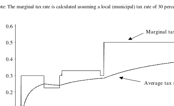
Households who are eligible for SA may also be eligible for HA, which is deter-mined by nation-wide benefit rules. The allowance is targeted at families with chil-dren. In 1993, households without children could qualify for HA, but a reform introduced in 1997 essentially eliminated that possibility.6Eligibility for HA benefits depends on household income, cost for housing, and the size of the household. In Figure 2, we show how HA changes with changes in family income for a household with two children. In 1993, the amount of HA a family receives is constant for incomes below SEK 90,000. For higher incomes, the benefits are reduced at a rate of 20 percent. In 1993, about 50-70 percent of the housing cost is covered by HA for a family with an income below SEK 90,000. As shown in Figure 2, HA benefits are less generous in 1999 compared with 1993. The structure of the HA system is the same, and the reduction rate is also similar. However, the income level after which benefits
6. However, single persons younger than 29 years old without children could still qualify for the allowance.
120000
Amount of Bene ts
100000
Social Assistance in 1993
Social Assistance in 1999
80000
60000
40000
20000
0
Net Income
0
20000 40000 60000 80000 100000 120000 140000 160000 180000 200000 220000 240000 260000 280000 300000
Figure 1
SA Benefits in Sweden, 1993 and 1999
are reduced is substantially lower, SEK 60,000 in 1999 compared with SEK 90,000 in 1993.
III. Income Taxes in Sweden
The Swedish income tax system is composed of two parts—a munic-ipal tax rate and a national tax rate. The national government determines the tax base for both national and local income taxes, but each municipality has the authority to set its own rate. In general, the same rules regarding exemptions and deductions apply, and individuals file only one return for both local and national taxes. Each resident with income above a certain threshold (SEK 11,008 in 1993 and SEK 8,736 in 1999) must file an income tax return. Further, the individual is the unit of taxation and income taxes are independent of household composition.
Although local taxes are proportional, the national income tax is progressive. There is a large variation in local taxes across municipalities. In 1993, the average tax rate
120000
Amount of Bene ts
100000
80000
60000
40000
20000
Housing Allowance in 1999
Housing Allowance in 1993
0
0
20000 40000 60000 80000 100000 120000 140000 160000 180000 200000 220000 240000 260000 280000 300000
Before Tax Income (Including transfers)
Figure 2
HA in Sweden, 1993 and 1999
was 30.95 percent with a minimum of 25.89 percent and a maximum of 33.80 per-cent. For 1999, the corresponding figures are 31.51 percent, 26.25 percent and 34.64 percent, respectively. A major tax reform in 1991 significantly reduced the national income tax rate and removed most of the tax brackets. In 1993, the national tax rate is essentially zero for incomes up to a threshold level of SEK 190,600 and it is 20 per-cent on incomes above that level.7 In 1999, the national income tax schedule had three income brackets: A zero tax rate for incomes up to SEK 219,300, a tax rate of 20 percent on incomes between SEK 219,300 and SEK 360,000, and a tax rate of 25 percent on incomes above SEK 360,000.
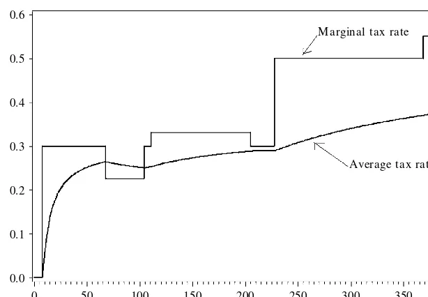
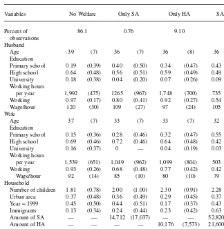
Despite the fact that most income earners are only paying local income taxes, which are proportional, there is variation in the marginal tax rates paid by these tax payers. Table 1 shows how the general deductions vary with taxable income evaluated at a municipal tax rate of 30 percent. In 1993, the marginal tax rate on incomes between SEK 11,000 and SEK 64,000 equals the municipal tax rate. However, between SEK 64,100 and SEK 99,500, the deductions from taxable income increase with income and the marginal tax rate is lower. In the example in Table 1, the marginal tax rate is 22.5 percent in this income bracket. For incomes between SEK 104,600 and SEK 193,000, the deductions are reduced as income increase and the marginal tax rate is higher than the municipal tax rate. The same pattern regarding the marginal income taxes is observed in 1999. Figures 3 and 4 illustrate how both the marginal and aver-age tax rate vary with taxable income. This peculiar shape of the marginal tax profile is most likely due to political considerations. During the 1991 tax reform, the national income tax rate was reduced significantly for high income earners while low-income earners were less affected by the reform. To compensate the latter group and to reduce the after-tax income inequality generated by the reform, additional deductions were allowed on incomes between certain levels.
IV. Economic Model and Empirical Specification
As mentioned above, the traditional way to model labor supply assumes that the decision variable, hours of work, is continuous. However, in this framework restrictive assumptions must be made in order to guarantee statistical coherency (see, for instance, the discussion in MaCurdy, Green, and Paarsch 1990). Moreover, an underlying assumption in traditional labor supply models is that the individual (or household) budget set is convex. Hence, to estimate such a model, a number of important simplifications of the income tax and transfer system must be made.
In this paper, we model labor supply as a discrete choice instead, following previ-ous work by van Soest (1995); Hoynes (1996); Keane and Moffitt (1998), and Blundell et al. (2000). Unlike the continuous labor supply model, the discrete choice model allow us to include as many details as possible regarding the budget set and it extends naturally into a household model, where husbands and wives jointly deter-mine their labor supply. Specifically, we assume that each household can choose
Figure 3
Income taxes in Sweden 1993
Note: Income taxes are evaluated at a municipal tax rate of 30 percent. 0.0
0.1 0.2 0.3 0.4 0.5 0.6
Taxable income-thousands of SEK
0 50 100 150 200 250 300 350 400
M arginal tax rate
Average tax rate Table 1
Description of the Swedish Income Tax System in 1993 and 1999
Marginal Tax Rate
Income Levels General Deductions (Percent)
1993
−10,900 All Income 0
11,000-64,000 11,000 30
64,100-99,500 11,000+0.25*(Income-64,100) 22.5
99,600-104,500 19,875 30
104,600-193,000 19,875-0.1*(Income-104,600) 33
193,100-201,500 11,000 30
201,600- 11,000 50
1999
−8,500 All Income 0
8,600-67,500 8,500 30
67,600-105,500 8,500+0.25*(Income-67,600) 22.5
105,600-110,500 20,200 30
110,600-203,500 20,200-0.1*(Income-110,600) 33
203,600-227,000 8,500 30
227,000-368,500 8,500 50
368,600- 8,500 55
among the alternatives in the choice set of income-leisure combinations (NIj,j¢, LHUSj,LWIFEj¢), where j =1,..., Jand j¢ =1,..., J. Further, LHUSj =TE-hhus,jand LWIFEj¢=TE-hwife,j¢where TEdenotes each spouse’s time endowment and is set to 4,000 hours per year.8Thus, the choice set for a household contains J2different hours of work combinations. In the empirical part of the paper, we set J =7.9
We assume that family utility depends not only on income and leisure, but also on participation in welfare programs. The two welfare programs considered in this paper are SA and HA. These, along with child allowance, are the main public cash assis-tance programs for two-parent families in Sweden. We do not model participation in child allowance since these benefits are paid automatically to parents and are inde-pendent of household income.
We further assume that the utility function is increasing in income and leisure and decreasing in welfare participation (SA and/or HA). The disutility from participation in a welfare program is assumed to primarily reflect the nonmonetary costs associated with participation in such programs, such as fixed costs or “stigma,” and is included to account for nonparticipation among eligible families.10
8. TEalso can be regarded as a parameter that can be estimated together with all other parameters. 9. We set hi,1=0, hi,2=500, hi,3=1000, hi,4=1500, hi,5=2000, hi,6=2500,and hi,7=3000for i=hus,wife. 10. What may appear as “stigma” or disutility from welfare participation may also result from the inability of the econometrician to measure true welfare eligibility. Moreover, imperfect information regarding benefit eligibility on behalf of the household is also included in this nonmonetary cost.
Figure 4
Income taxes in Sweden 1999
Note: Income taxes are evaluated at a municipal tax rate of 30 percent. 0.0
0.1 0.2 0.3 0.4 0.5 0.6
Taxable income-thousands of SEK
0 50 100 150 200 250 300 350 400
M arginal tax rate
Following van Soest (1995), we use a trans-log specification of the direct utility function, and for any specific household we have:
( )
U NI LHUS LWIFE NI LHUS LWIFE
NI LHUS LWIFE
where j=1,...,Jand j¢=1,...,Jand where it is assumed that the disutility from receiving SA(φSA) and from receiving HA (φHA) is separable from the utility of leisure and dis-posable income (following Moffitt 1983 and Hoynes 1996).
The household choose LHUS, LWIFE, dSA, dHAand consumption (or net income) by maximizing family utility subject to the following budget constraint:
j ( , )
HA hus wife HA hus wife
l
where NIj,husand NIj¢,wifeare the income net of taxes for husbands and wives at hours combinations j and j¢, respectively. BSA(.,.) is the amount of household specific SA
benefits, BHA(.,.)is the amount of household specific HA and CC(.,.)represents child-care costs. BSA(.,.), BHA(.,.), and CC(.,.)all depend on family income. Further, CC(.,.), as well BSA(.,.)prior to January 1998, are determined at local (municipal) levels. The individual components to household net income are given as:
( ) ( )
j wife wife j wife wife wife j wife wife
T
j wife
= + - +
-= + - +
-l l l l
where Wequals the before-tax hourly wage rate, his annual hours of work, Ydenotes annual nontaxable, nonlabor income, t(.)is a function that determines income taxes, YTis taxable nonlabor income, and Drepresents deductions.11
The addition of the disutility of welfare participation implies that a family faces 4*J2work-welfare possibilities (neither SA nor HA, SA but not HA, HA but not SA, and both SA and HA). Some welfare states may be infeasible if the household income from work is sufficiently high to render them ineligible for SA and/or HA. Solving the optimization problem requires evaluating the utility function in Equation 1, for each possible combination of husband’s hours, wife’s hours, welfare program partic-ipation, and choosing the state that yields the highest utility.
In order to empirically implement the model, we need to specify the nature of hetero-geneity in household preferences and the stochastic disturbances. Heterohetero-geneity in preferences for leisure and welfare is introduced as
1
1
where the elements of the vectors xand zare observed individual and family charac-teristics, such as age and education of both spouses and the number and ages of chil-dren. Kxand Kzdenote the dimensions of the vectors xand z, respectively, while the
θs represent unobserved variables that affect preferences for leisure and welfare. It is reasonable to assume that an important source for population heterogeneity in terms of preferences for leisure and welfare is unobserved. In order to account for this, we formulate a finite mixture model, which allows for unobserved heterogeneity in a flexible way without imposing a parametric structure. This way of representing unobserved heterogeneity is similar to what Heckman and Singer (1984) suggested for duration data models. We assume that there exist Mdifferent sets of θ, {θhus, θhussq,
θwife, θwifesq, θSA, θHA}, that determine a family’s preferences, each observed with prob-ability πm(where πm>0 and Σπm=1, m =1,...,M). This specification allows for arbi-trary correlations between the husband’s and the wife’s work effort as well as between each spouse’s work effort and preference for welfare participation.
To make the model estimable, additional random disturbances are added to the utilities of all choice opportunities:
( )5 Uj j r, ,l =U NI( j j,l,LHUS LWIFEj, jl)+fj j r, ,l
where j (=1,...,J)represents the husband’s choice of labor supply, j¢(=1,...,J)
repre-sents the wife’s choice of labor supply, and r (=1,...,4)represents the household’s wel-fare participation state, and denotes the household utility of choice (j,j¢,r). We assume
that εj,j¢,rfollows a Type Iextreme value distribution with cumulative density Pr(εjj¢,r<ε)
=exp(−exp(−ε)). The error term εj,j¢,rcan be interpreted as an unobserved alternative specific utility component or as an error in a household’s assessment of the utility associated with choosing the work-welfare combination (j,j¢,r)(optimization error).
Thus, it has a different interpretation compared with the θs introduced above, which represents unobserved preferences for leisure and welfare. Given the distributional assumptions of the stochastic terms in the utility function, the contribution to the likelihood function for a given household is
and where Θ = {θhus, θhussq, θwife, θwifesq, θSA, θHA} and dj,j¢,ris an indicator for the
observed state for each household. This expression simply denotes the probability that the utility in state (j,j¢,r)is the highest among all possible work-welfare combinations,
conditional on unobserved preferences.
The discrete state labor supply model requires a rule for mapping a continuum of hours of work into a finite number of classes. There is no obvious way of transform-ing continuous hours into discrete categories and the results may be sensitive to the rule used to assign the discrete states.12In this paper, we try to limit the possibility of aggregation errors in hours of work by using a multiplicative classification error spec-ification, following MaCurdy, Green, and Paarsch (1990) and Hoynes (1996).13 Let Hhusand Hwifedenote reported hours and hhusand hwifeoptimal (discrete) hours. The multiplicative classification error specification is given as
( )7 Hi hiexp( )i with i N( 21 i, i)fori hus wife,
2 2 +
= h h - v v =
This design for the classification error implies that zero hours are observed with certainty, but when optimal hours are positive, they differ from reported hours by a factor of proportionality. As discussed in Hoynes (1996), this is not a measurement error in the traditional sense. Instead, this error measures the difference between reported hours and the discrete representation of hours (Hhus−hj,husfor the husband and Hwife−hj¢,wifefor the wife). Thus, it can be regarded as a “within group” error and it essentially gives more weight to groups where this “within group” error is small.
The assumptions presented in Equation 7 above implies that the density functions for the “within group” errors are
( )
12. This may be especially true for women as the distribution of hours of work for this group shows a considerably higher variance than the corresponding distribution for men.
In presence of unobserved heterogeneity and “within group” errors, the contribution to the likelihood function for a given household is represented by
1 1 1 1
( )9 l
冱
冱 冱 冱
(p| ), , g, g , , ,M m
J J
j j r j hus j wife j j r
4
= r H l l d l
= r= j= =
m * jl 4
where gj,husand gj¢,wifeare defined in Equation 8 above.
V. Data
A. Description of the Data and Sampling Procedures
The data used in this paper are taken from the Swedish Income Distribution Survey (HEK). This is an annual survey conducted by Statistics Sweden and it contains infor-mation on labor market activities, demographic characteristics, and incomes for a ran-dom sample of Swedish individuals. Information is also collected for their household members. The survey was initiated in 1975. The second survey took place in 1978; since 1980 Statistics Sweden has conducted annual surveys. Each survey is a cross-sectional representative of the population and in this paper we pool data from the 1993 and 1999 surveys. The reason for choosing these two surveys is that they represent times of recession (1993) and economic growth (1999). Another reason is that this provides us with data from before and after the changes in the SA benefit rules.
Information on individuals and households is obtained from three sources: vari-ous government registers, a phone interview, and income tax returns. Data on incomes, wages, transfers, taxes, wealth, and educational attainments are collected from different government registers whereas information on capital gains or losses is obtained from income tax returns. During the phone interviews, respondents are asked about individual and family characteristics, such as marital status, age and number of children, labor supply, childcare expenses, and cost of living. We have supplemented the information in the surveys with data from the Swedish munici-palities who provided information on SA benefit levels. As mentioned above, in 1993, the levels depend on the municipality in which the household resides, as well as on the family composition, such as marital status, age, and number of children. In 1999, the benefit levels depend only on family composition and not on geo-graphical location.
The sample used for estimation includes families that satisfy the following selec-tion criterion: (i) family contains a married or cohabitant couple with at least one child younger than 18 in the household, (ii) family has no taxable wealth, (iii) the house-hold’s nonlabor income is less than the SA benefit level, and (iv) both parents must be younger than 56 years old.14In addition to these selections, we also excluded fam-ilies where one or both parents were either full-time students, retired, or self-employed. The reason for these sample selections is that they retain families who, apart from their labor income, are eligible for both SA and HA.
B. Variable Definitions
As mentioned above, information on income in HEKis obtained from administrative records with precise information on earnings and nonlabor income. The wage data were collected from the Official Statistics on Wages produced by Statistics Sweden, which are based on employers’ reports of individual wages.15 These data have the advantage over the usual self-reported wage data of being free from recall error. The wage data cover all employed persons in the public sector and parts of the private sec-tor. For the private sector, Statistics Sweden took a random sample of firms and col-lected wages for workers in the secol-lected firms. To account for missing wages among nonworkers, log wage equations for husbands and wives are estimated accounting for potential sample selection bias. In order to be consistent regarding the stochastic spec-ification, the wage equation estimates are used to predict wages for both workers and nonworkers.16
Nonlabor income includes income from capital gains, child allowance and child support payments. Unemployment benefits and other transfers that depend on labor supply are excluded from our measure of nonlabor income. We allow the general deductions that depend on labor supply, as shown in Table 1, to vary with hours of work. Other income-dependent deductions have been excluded.
To generate net income for different combinations of hours of work, we use a microsimulation model (FASIT).17The micro simulation model contains very precise information on income tax rules as well as on eligibility rules for a number of welfare programs, such as SA and HA. In addition, FASIT also enables us to calculate the childcare cost for each combination of hours of work. Access to a simulation model such as FASIT is essential in order to calculate accurate (net) incomes for a given household, conditional on labor supply, as the income tax system and the benefit lev-els for different welfare programs are complicated functions of earnings and nonlabor income.
Information on labor supply is obtained during the phone interview. Respondents are asked about hours of work, for each month, including overtime. This definition is consistent with the earnings information provided by the employer. Regarding wel-fare participation, there is register information on the number of months a household received SA (as well as the amount received) in HEK.18However, we are not able to determine in which month(s) a household received the benefit. This implies that we are not able to use monthly data in the analysis. Instead we must aggregate all
infor-15. The employers reported monthly earnings information to Statistics Sweden. The earnings figures are expressed in full-time equivalents and give the amount the individual would have earned had he or she worked full time. To obtain full-time equivalent hourly wage rates, the monthly earnings are divided by 165. 16. Using predicted wages for both workers and nonworkers implies that the budget set is not perfectly observed. An alternative is to use observed wages for workers and predicted wages for nonworkers. However, this may produce bias in the estimates as this could introduce spurious differences in wage distributions across the two groups.
17. FASIT is used and developed by Statistics Sweden and the Swedish Ministry of Finance. A similar microsimulation model exists for the U.K. (TAXBEN).
mation to an annual basis.19 Thus, a household is defined as a SA recipient if it received some assistance for at least one month during the year. Most of the SA households received benefits for a short period. Of all the SA recipients, about 50 per-cent received it for three months or less and about 20 perper-cent for more than seven months. There is also register information on the amount of HA each house-hold received in a given year. We created binary variables (dSAand dHA) indicating participation status in SA and HA, respectively.
The variables that are included in the xand zvectors (which determine observed heterogeneity in distaste for work and welfare) are: age, education of the husband and the wife where education is measured by two dummy variables describing the high-est grade completed (high school and college/university), number of children, a dummy variable for youngest child younger than three years old, a dummy variable for youngest child aged three to six, a dummy variable indicating the immigrant sta-tus of the household (a household is defined to be an immigrant household if the hus-band and/or the wife was born abroad), a dummy variable that equals one if the household resides in any of the three largest cities in Sweden (Stockholm, Goteborg, Malmo) and finally a time dummy variable which equals one for 1999.
C. Descriptive Statistics
Table 2 shows descriptive statistics for the sample used in this study by welfare par-ticipation status. All wage and benefit variables are measured in 1999 SEK using the consumer price index to adjust the 1993 values. Of the total 3,297 families, 25 (0.76 percent) received only SA, 300 (9.1 percent) received only HA, while 134 (4.06 per-cent) received both SA and HA. Households receiving any of the welfare programs considered in this paper are younger, less educated and work less than those not receiving SA or HA. The hourly wage rate is also lower among welfare recipients. Moreover, families receiving welfare have more children and are to a greater extent defined as immigrant households. The average amount of assistance or allowance received, among participants, is SEK 14,712 per year for SA and SEK 10,176 per year for HA. For families that receive both SA and HA, the average amounts are SEK 52,820 per year for SA and SEK 21,600 per year for HA.
VI. Results
A. Structural Estimates
The estimated parameters of the structural model associated with observable charac-teristics are presented in Table 3. Before discussing the implications of these esti-mates, it is worthwhile noting that the utility function—evaluated at these estimates and at observed hours of work and disposable income—fulfills the conditions for
quasi-concavity for virtually all households (the condition was rejected for only 22 households out of 3,297). Because there is a fair amount of variation in both hours of work and disposable income, this suggests that the utility function is concave over a large region. Given that the estimated utility function satisfies the theoretical requirements, we can use it for predictions and simulations.
The last two columns in Table 3 present results that refer to the disutility associated with SA participation (Column 5) and with receiving HA (Column 6). In both cases, a positive sign of a coefficient implies that the disutility of participation in a particu-lar welfare program is increasing in that variable since both zSAand zHAenters nega-tively in the utility function. The estimates suggest that the disutility of both welfare Table 2
Sample Averages by Welfare Status (N =3,297)
Variables No Welfare Only SA Only HA SA and HA
Percent of 86.1 0.76 9.10 4.06
observations Husband
Age 39 (7) 36 (7) 36 (8) 36 (9)
Education
Primary school 0.19 (0.39) 0.40 (0.50) 0.34 (0.47) 0.43 (0.50) High school 0.64 (0.48) 0.56 (0.51) 0.59 (0.49) 0.49 (0.50) University 0.18 (0.38) 0.04 (0.20) 0.07 (0.26) 0.09 (0.29) Working hours
per year 1,992 (475) 1265 (967) 1,748 (700) 735 (859) Working 0.97 (0.17) 0.80 (0.41) 0.92 (0.27) 0.54 (0.50)
Wage/hour 120 (30) 109 (27) 97 (24) 105 (32)
Wife
Age 37 (7) 33 (7) 33 (7) 32 (7)
Education
Primary school 0.15 (0.36) 0.28 (0.46) 0.32 (0.47) 0.55 (0.50) High school 0.69 (0.46) 0.72 (0.46) 0.64 (0.48) 0.42 (0.50) University 0.16 (0.37) 0 — 0.04 (0.19) 0.03 (0.17) Working hours
per year 1,539 (651) 1,049 (962) 1,099 (804) 503 (749) Working 0.93 (0.26) 0.68 (0.48) 0.77 (0.42) 0.42 (0.50)
Wage/hour 92 (14) 85 (10) 80 (10) 79 (13)
Household
Number of children 1.81 (0.78) 2.00 (1.00) 2.30 (0.91) 2.28 (1.20) Urban area 0.37 (0.48) 0.36 (0.49) 0.29 (0.45) 0.37 (0.48) Year =1999 0.45 (0.50) 0.44 (0.51) 0.17 (0.37) 0.43 (0.50) Immigrants 0.13 (0.34) 0.24 (0.44) 0.23 (0.42) 0.63 (0.48) Amount of SA — — 14,712 (17,037) — — 52,820 (49,432) Amount of HA — — — — 10,176 (7,573) 21,600 (12,182) Total amount of
welfare — — 14,712 (17,037) 10,176 (7,573) 74,420 (57,456) Number of
observations 2,838 25 300 134
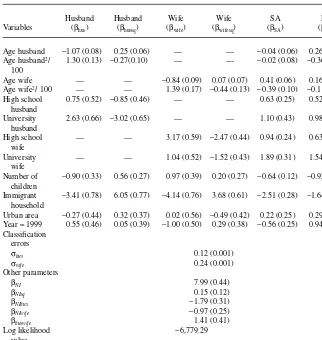
programs increase with age (at a decreasing rate) and education, decrease with number of children and is lower among immigrant households.
Because of the nonlinear nature of the model with respect to labor supply, the mag-nitudes of the coefficient estimates provide little information about the size of the effects of the observable characteristics. Therefore, instead of discussing the coeffi-cient estimates that are reported in Columns 1–4 in Table 3, we present the percent-age changes in hours of work associated with changes in observed characteristics for a representative (using the modes of observable characteristics) husband and wife, Table 3
Estimates of a Structural Household Labor Supply Model: Effects of Observed Heterogeneity and of Classification Errors
Husband Husband Wife Wife SA HA
Variables (βhus) (βhussq) (βwife) (βwifesq) (βSA) (βHA)
Age husband −1.07 (0.08) 0.25 (0.06) — — −0.04 (0.06) 0.26 (0.02) Age husband2/ 1.30 (0.13) −0.27(0.10) — — −0.02 (0.08) −0.36 (0.03)
100
Age wife — — −0.84 (0.09) 0.07 (0.07) 0.41 (0.06) 0.16 (0.02) Age wife2/ 100 — — 1.39 (0.17) −0.44 (0.13) −0.39 (0.10) −0.11 (0.03)
High school 0.75 (0.52) −0.85 (0.46) — — 0.63 (0.25) 0.52 (0.15) husband
University 2.63 (0.66) −3.02 (0.65) — — 1.10 (0.43) 0.98 (0.26) husband
High school — — 3.17 (0.59) −2.47 (0.44) 0.94 (0.24) 0.63 (0.15) wife
University — — 1.04 (0.52) −1.52 (0.43) 1.89 (0.31) 1.54 (0.32) wife
Number of −0.90 (0.33) 0.56 (0.27) 0.97 (0.39) 0.20 (0.27) −0.64 (0.12) −0.92 (0.08) children
Immigrant −3.41 (0.78) 6.05 (0.77) −4.14 (0.76) 3.68 (0.61) −2.51 (0.28) −1.64 (0.15) household
Urban area −0.27 (0.44) 0.32 (0.37) 0.02 (0.56) −0.49 (0.42) 0.22 (0.25) 0.29 (0.14) Year =1999 0.55 (0.46) 0.05 (0.39) −1.00 (0.50) 0.29 (0.38) −0.56 (0.25) 0.94 (0.15) Classification
errors
σhus 0.12 (0.001)
σwife 0.24 (0.001)
Other parameters
βNI 7.99 (0.44)
βNIsq 0.15 (0.12)
βNIhus −1.79 (0.31)
βNIwife −0.97 (0.25)
βhuswife 1.41 (0.41)
Log likelihood −6,779.29
value
Number of 3,297
observations:
respectively. The results are shown in Table 4. For husbands, the effects of number of children, education, and region of living (rural versus urban area) on labor supply are small (the changes range from 0.01 percent to 0.04 percent in absolute terms). The largest labor supply responses are associated with changes in: immigrant status, where the estimates imply fewer hours worked for men in immigrant households; time, the estimates suggest that hours of work is less in 1999 compared with 1993; and finally for age, where hours worked increase with age. For wives, the effects of all observable variables are larger in absolute terms, and hours of work is negatively associated with number of children and immigrant status, and positively associated with education, region of living, time, and age. Overall, the signs and the magnitudes of these effects on labor supply are as expected.
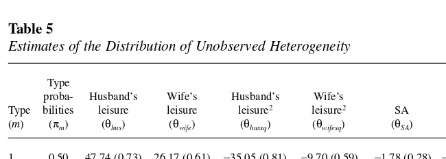
The estimates of the distribution of the unobserved heterogeneity components are shown in Table 5. Because unobserved heterogeneity enters both in βhusand βhussq(as Table 4
Percentage Changes in Hours of Work Associated with Changes in Observed Characteristics for a Representative Husband and Wife
Variable Husband Wife
Increase the number of children from two to three 0.04 −3.03
Increase husband’s education from high school to university 0.04 −0.02
Increase wife’s education from high school to university 0.01 2.21
Immigrant household as opposed to a native household −1.49 −4.45
Living in an urban area as opposed to living in rural areas 0.01 1.38
1999 instead of 1993 −0.26 1.48
Increase husband’s age from 36 to 37 0.27 0.04
Increase wife’s age from 35 to 36 0.01 0.72
Table 5
Estimates of the Distribution of Unobserved Heterogeneity
Type
proba- Husband’s Wife’s Husband’s Wife’s
Type bilities leisure leisure leisure2 leisure2 SA HA
(m) (πm) (θhus) (θwife) (θhussq) (θwifesq) (θSA) (θHA)
1 0.50 47.74 (0.73) 26.17 (0.61) −35.05 (0.81) −9.70 (0.59) −1.78 (0.28) −5.48 (0.17) 2 0.05 28.24 (1.69) 23.03 (1.17) −5.97 (0.90) −11.64 (1.21) −5.13 (0.27) −6.70 (0.26) 3 0.26 50.25 (0.83) 20.71 (1.11) −49.13 (1.74) −0.88 (0.62) 10.95 (0.01) −5.41 (0.23) 4 0.09 26.66 (0.86) 18.74 (1.82) −8.22 (0.76) 0.07 (0.83) −5.71 (0.33) −7.93 (0.27) 5 0.05 32.86 (0.74) 59.21 (0.43) −18.56 (0.67) −6.49 (1.17) −5.06 (0.28) −7.21 (0.25) 6 0.05 49.53 (0.52) 20.77 (1.32) −22.04 (0.57) −6.00 (1.15) 10.33 (0.01) 7.99 (0.01)
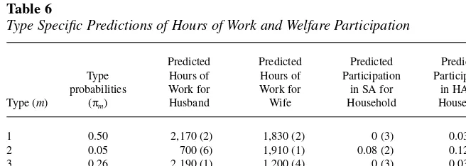
well as in βwifeand βwifesq) it is not obvious which types have strong preferences for leisure and which types have not. To illustrate the variation in hours of work and in welfare participation due to unobserved heterogeneity, we obtained type-specific pre-dictions of hours of work and participation in SA and HA. That is, we first assumed that every household in the sample has the unobserved preference structure of Type 1 families and predicted outcomes based on this. This was repeated for all six types and the results, along with type-specific rankings, are shown in Table 6. The entries in this table show that in households of Type 1, which make up about 50 percent of the sam-ple, both husbands and wives have strong preferences for work (predicted hours of work ranks second for both husbands and wives). This household type also receives a strong disutility from participation in either SA or HA, indicated by the low predicted participation rates in each program for this family type. The second household type shows families where the husband has weak preferences for work while the wife has strong preferences for work, while the opposite holds for Type 3 families. In Type 4 and Type 6 families, both spouses have weak preferences for work while in Type 5 households, only the wife has weak preferences for work. The household type that appears most likely to participate in SA and/or HA is Type 4 (ranked first in both SA and HA), followed by Type 5 and Type 2.
The specification used for the distribution of unobserved heterogeneity allows for unrestricted correlations between unobserved preferences for work for the husband (determined by both θhusand θhussq), for the wife (determined by θwifeand θwifesq) as well as for the household’s preferences for welfare participation (θSAand θHA). The empirical correlation coefficient between the husband’s and the wife’s unobserved preference for work is -0.05. This suggests that, holding observable characteristics constant, higher work effort for the husband is associated with lower work effort for the wife. Regarding the correlation between the unobserved elements of work effort and welfare participation, the results indicate strong negative correlations both for husbands and wives. For husbands, the empirical correlation coefficient between work effort and participation in SA is −0.68 and it is −0.52 between work effort and partic-ipation in HA. For wives, the corresponding figures are −0.51 and −0.58, respectively.
Table 6
Type Specific Predictions of Hours of Work and Welfare Participation
Predicted Predicted Predicted Predicted Type Hours of Hours of Participation Participation probabilities Work for Work for in SA for in HA for
Type (m) (πm) Husband Wife Household Household
1 0.50 2,170 (2) 1,830 (2) 0 (3) 0.03 (4)
2 0.05 700 (6) 1,910 (1) 0.08 (2) 0.12 (3)
3 0.26 2,190 (1) 1,200 (4) 0 (3) 0.03 (4)
4 0.09 1,520 (5) 1,020 (5) 0.13 (1) 0.32 (1)
5 0.05 2,150 (3) 0 (6) 0.08 (2) 0.21 (2)
6 0.05 1,670 (4) 1,800 (3) 0 (3) 0 (6)
Negative correlations between work effort and welfare participation was also found by Hoynes (1996) and suggest existence of self-selection into welfare programs.
B. Model Fit
A common problem in many labor supply studies is the poor ability to fit the observed distribution of hours of work. One option to improve the ability of the estimated model to mimic the observed frequencies of hours of work is to try to control for unobserved fixed costs of work (see, for example, Kapteyn, Kooreman; van Soest 1990; and van Soest 1995). Alternatively, we can specify a flexible model with respect to unobserved heterogeneity, which may to some extent represent unobserved fixed costs of work as well as unobserved preferences for leisure, to improve the model fit. This is the approach taken in this paper and, as can be seen in Table 7, the predicted distribution of hours is quite similar to the observed distribution, both for men and for women.
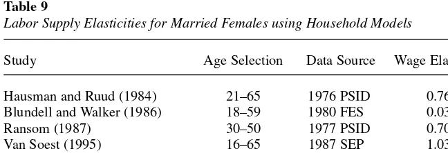
C. Elasticities
The effects of wage changes are assessed using simulations. Specifically, wages were increased by 10 percent for everyone in the sample and the resulting changes in pre-dicted working hours were calculated. The results imply that working hours are quite insensitive to wage changes, especially for males. For instance, a 10 percent wage increase for husbands, holding everything else constant, is associated with an average increase in hours of work equal to 0.5 percent. For women, the corresponding labor supply response is an increase by 1 percent. A wage inelastic labor supply for men is not uncommon in the literature, regardless of model specification and data source. The entries in Table 8 show estimated uncompensated wage elasticities obtained using structural household labor supply models and they range from −0.04 to 0.15. Thus, Table 7
Observed and Predicted Hours of Work Frequencies (in percentages)
Husband’s Husband’s Wife’s Wife’s
Observed Predicted Observed Predicted
Hours Category (hj) Distribution Distribution Distribution Distribution
h1=0 5.16 6.67 11.13 15.01
h2=500 1.09 0.45 4.76 2.0
h3=1000 2.49 1.88 4.34 3.61
h4=1500 2.94 1.88 15.59 8.58
h5=2000 6.55 5.91 27.57 44.16
h6=2500 77.37 82.04 36.0 26.6
h7=3000 4.40 1.15 0.61 0.03
our results for husbands are quite similar to those found previously in the literature. For women, the existing literature shows more variation in terms of the labor supply response to wage changes. In Table 9, we summarize the results from a selection of such studies, again focusing on structural household labor supply models. The esti-mated elasticities range from 0 to 1.03, depending on model specification and data source, and our results for women are generally lower than most of the existing results.
D. Policy Simulations
To illustrate the effects on labor supply of changes in income taxes and in benefit rules for both SA and HA, we performed a simple simulation experiment. In Sweden, as well as in many other countries, there is a concern about the high implicit marginal tax rates of an increase in working hours for low-income families. These effects are Table 8
Male Labor Supply Elasticities for Married Males using Household Models
Study Age Selection Data Source Wage Elasticity
Hausman and Ruud (1984) 21–65 1976 PSID −0.03
Blundell and Walker (1986) 18–59 1980 FES 0.02
Ransom (1987) 30–50 1977 PSID −0.04
Van Soest (1995) 16–65 1987 SEP 0.15
Van Soest and Das (2001) 16–64 1995 SEP 0.08
Bonin, Kempe, and Schneider 18–60 2000 GSEP 0.00
(2002)
Note: PSID=US Panel Study of Income Dynamics, FES =UK Family Expenditure Survey, SEP=Dutch Socio-Economic Panel, GSOEP=German Socio-Economic Panel.
Table 9
Labor Supply Elasticities for Married Females using Household Models
Study Age Selection Data Source Wage Elasticity
Hausman and Ruud (1984) 21–65 1976 PSID 0.76
Blundell and Walker (1986) 18–59 1980 FES 0.03
Ransom (1987) 30–50 1977 PSID 0.70
Van Soest (1995) 16–65 1987 SEP 1.03
Van Soest and Das (2001) 16–64 1995 SEP 0.71
Bonin, Kempe, and Schneider 18–60 2000 GSEP 0.00
(2002)
mainly due to the existence of a relatively high income tax rate on low earnings com-bined with a high implicit tax on welfare benefits. To investigate the labor supply effects of a reduction of these strong work disincentive effects for low-income fami-lies, we used our estimates to predict hours of work during the current tax and trans-fer system as well as during a modified system. Specifically, we increased the general deductions from SEK 11,000 to SEK 68,800 in 1993 and from SEK 8,500 to SEK 72,800 in 1999, which substantially lowers income taxes for all families, but relatively more for low-income households. We also reduced the benefit levels for both SA and HA with 25 percent as additional labor supply incentives.
As a result of the suggested tax and benefit changes, working hours increase on average by 1.1 percent for wives and by 0.3 percent for husbands. Further, disposable or net income increase by almost 12 percent and income tax revenues decrease by 28 percent. As expected, the policy change has a dramatic effect on government spend-ing on both SA (a reduction with 44 percent) and HA (a reduction with 28 percent) but the effects on participation in these programs are limited. Despite the strong reduction in income tax rates and the substantially reduced welfare benefit levels, the average effects on labor supply are quite small. This demonstrates the difficulties associated with financing any reform that implies a large reduction in income taxes.20 In fact only 0.6 percent of the husbands and 2.0 percent of the wives change their working hours in response to the policy change. This is a natural consequence of the discrete approach to modeling labor supply where the dominating prediction is no change in working hours.
A more detailed presentation of the changes in labor supply, disposable income and income taxes for the whole sample is given in Table 10. This table also shows the wel-fare effects of the reform. We chose EV as our money metric of a welwel-fare change. EV is measured as the amount of money added or subtracted from the households’ dis-posable income under the initial tax rules in order to make the household indifferent between the initial and the alternative tax system. As such, EV summarizes the household’s net welfare change associated with behavioral responses.
The average EV for the whole sample is SEK 36,169. However, there is a substan-tial variation across households. Table 10 lists EV for different levels of prereform disposable income. The estimated average EV for the poorest 10 percent is SEK 11,345 per year compared with SEK 57,195 per year for the richest 10 percent.
As mentioned above, the average effects of the tax reduction on working hours were relatively small. However, this does not imply that the effects for all income groups are small. Table 10 presents the predicted changes in working hours for dif-ferent prereform income groups. The results suggest a relatively strong increase in both the wife’s and the husband’s hours of work (8 percent and 3 percent, respec-tively) among low-income households. However, and as expected, among the richest 10 percent there are virtually no changes in labor supply.
To summarize, a reduction in income taxes and welfare benefits has considerable welfare effects and the difference in these effects between poor and rich households is substantial. The effect on working hours is, however, quite small and the policy change is associated with a sharp decline in income tax revenues.
E. Results from Alternative Specifications
This subsection examines the robustness of our results to different model assumptions as well as to a different definition of SA participation. Regarding alternative model specifications, we consider a naïve model with no unobserved heterogeneity or wel-fare stigma, a model with no observable characteristics affecting βhussq, βwifesq, zSAand
zHA, and finally a model where we include observed and unobserved heterogeneity in
βNIinstead of in βhussqand βwifesq. To assess the effects of wage changes on labor sup-ply, we again increased wages by 10 percent and the resulting changes in predicted working hours were calculated. For husbands, we find that a 10 percent wage increase is associated with increases in hours of work ranging from 0.1 percent to 0.4 percent, depending on model specification, which should be compared with 0.5 percent obtained in our preferred specification. For women, the corresponding labor supply responses using the alternative specifications range from 1.2 percent to 2.5 percent, somewhat higher than the 1 percent reported above.
Table 10
Results from a Tax and Transfer Simulation
Whole Sample Poorest 10 percent Richest 10 percent
Variable Husbands Wives Husbands Wives Husbands Wives
Working hours before 2,031 1,518 856 493 2,245 2,031
policy change
Working hours after 2,038 1,535 883 531 2,245 2,035
policy change
Disposable income 322,787 132,364 564,448
before policy change
Disposable income 360,388 147,536 621,634
after policy change
Income taxes paid 99,840 34,391 218,169
before policy change
Income taxes paid 71,854 19,318 180,095
after policy change
EV 36,169 11,345 57,195
In another attempt to explore the robustness of our results, we reestimated the model presented in Section IV using a different definition of SA participation. In the above analysis, a household is recorded as a SA participant if it received SA for at least one month during the year. This definition is arguably ad-hoc, and to verify that our results are not driven by our assignment rule for SA participation, we reestimated the model but with the difference that households are recorded as participants in SA only if they received payments for at least fourmonths during the year. The labor sup-ply effects from wage changes using this new definition on SA are similar to the ones reported above, with an increase in husbands and wives hours of work with 0.4 per-cent and 0.7 perper-cent, respectively. Overall, we find that the results and model impli-cations are quite robust toward both changes in model specification and to alternative variable definitions.
VII. Conclusions
In this paper, we used a sample of Swedish households with detailed and unique information on incomes and benefits and estimated a structural household labor supply model. We formulated a model where labor supply and participation in two welfare programs (SA and HA) were jointly determined. Further, the labor sup-ply and welfare participation decisions were treated as a discrete choice problem, and we assumed that these choices follow a simple conditional logit rule. We used a micro simulation model that incorporates many details of existing tax and government trans-fer system to calculate disposable income for diftrans-ferent work-welfare combinations. In addition, we allowed for unobserved individual-specific effects and for the possibility that these effects are correlated across alternatives. Classification errors in hours of work were allowed for by using a multiplicative classification error specification. The estimates from the structural model yielded small wage elasticities, both for husbands and wives. The result for men is similar to what earlier studies have reported, while our result for women is generally lower. We also performed a simple simulation experiment where we changed both the income tax structure and the benefit rules for SA and HA. The results from the policy simulation indicate that reducing income taxes significantly for low-income families along with a substantial reduction of max-imum welfare benefit levels generate substantial welfare effects. Using EV as our measure of the welfare effect associated with the tax and welfare change, we find that there are welfare gains for virtually everyone from the tax and transfer change. However, there are dramatic differences in EV depending on the level of prereform household income. The estimated average EV for the poorest 10 percent is SEK 11,345 per year compared with SEK 57,195 per year for the richest 10 percent.
References
Andren, Thomas. 2003. “The Choice of Paid Childcare, Welfare, and Labor Supply of Single Mothers.” Labour Economics10(2):133–47.
Blundell, Richard, Alan Duncan, Julian McCrae, and Costas Meghir. 2000. “Evaluating In-Work Benefit Reform: the In-Working Families Tax Credit in the UK.” London: Institute for Fiscal Studies. Unpublished.
Blundell, Richard, and Thomas MaCurdy. 1999. “Labor Supply: A Review of Alternative Approaches.” In Handbook of Labor Economics, Vol. 3, eds. Ashenfelter, Orley and David Card, 1559–1694. New York, NY: Elsevier Science Press.
Blundell, Richard, and Ian Walker. 1986. “A Life-Cycle Consistent Empirical Model of Family Labour Supply Using Cross-Section Data.” Review of Economic Studies 53(4):539–58.
Bonin, Holger, Wolfram Kempe, and Hilmar Schneider. 2002. “Household Labor Supply Effects of Low-Wage Subsidies in Germany.” Discussion Paper No. 637, Bonn: Institute for the Study of Labor.
Flood, Lennart, and Nizamul Islam. 2003. “Continuous or Discrete Dependent Variable? A Monte Carlo Comparison of Two Approaches,” Working Paper, Göteborg: Department of Economics, Göteborg University.
Flood, Lennart, Elina Pylkkanen, and Roger Wahlberg. 2003. “Labor Supply and Welfare Participation of Single Mothers in Sweden,” Working Paper, Göteborg: Department of Economics, Göteborg University.
Gong, Xiaodong, and Arthur van Soest. 2002. “Family Structure and Female Labor Supply in Mexico City.” Journal of Human Resources37(1):163–91.
Hagstrom, Paul. 1996. “The Food Stamp Participation and Labor Supply of Married Couples.” Journal of Human Resources31(2):383–403.
Hausman, Jerry. 1985. “The Econometrics of Nonlinear Budget Sets.” Econometrica 53(6):1255–82.
Hausman, Jerry, and Paul Ruud. 1984. “Family Labor Supply with Taxes.” American Economic Review74(2):242–48.
Heckman, James, and Burton Singer. 1984. “A Method for Minimizing the Distributional Assumptions in Econometric Models for Duration Data.” Econometrica52(2):271–320. Hoynes, Hilary. 1996. “Welfare Transfers in Two-Parent Families: Labor Supply and Welfare
Participation under AFDC-UP.” Econometrica64(2):295–332.
Kapteyn, Arie, Peter Kooreman, and Arthur van Soest. 1990. “Quantity Rationing and Concavity in a Flexible Household Labor Supply Model.” Review of Economics and Statistics72(1):55–62.
Keane, Michael, and Robert Moffitt. 1998. “A Structural Model of Multiple Welfare Program Participation and Labor Supply.” International Economic Review39(3):553–89.
MaCurdy, Thomas, David Green, and Harry Paarsch. 1990. “Assessing Empirical Approaches for Analyzing Taxes and Labor Supply.” Journal of Human Resources25(3):415–90. Levy, Frank. 1979. “The Labor Supply of Female Household Heads, or AFDC Work
Incentives Don’t Work Too Well.” Journal of Human Resources14(1):76–97.
Moffitt, Robert. 1983. “An Economic Model of Welfare Stigma.” American Economic Review 73(5):1023–35.
———. 1986. “Work Incentives in the AFDC System: An Analysis of the 1981 Reforms.” American Economic Review76(2):219–23.
———. 1992. “Incentive Effects of the U.S. Welfare System: A Review.” Journal of Economic Literature30(1):1–61.
Ransom, Michael. 1987. “An Empirical Model of Discrete and Continuous Choice in Family Labor Supply.” Review of Economics and Statistics69(3):465–72.
Van Soest, Arthur. 1995. “Structural Models of Family Labor Supply.” Journal of Human Resources30(1):63–88.