Real-Time Digital
Signal Processing
Implementations and Applications
Second Edition
Sen M Kuo
Northern Illinois University, USA
Bob H Lee
Ingenient Technologies Inc., USA
Real-Time Digital
Signal Processing
Implementations and Applications
Second Edition
Sen M Kuo
Northern Illinois University, USA
Bob H Lee
Ingenient Technologies Inc., USA
West Sussex PO19 8SQ, England
Telephone (+44) 1243 779777
Email (for orders and customer service enquiries): [email protected] Visit our Home Page on www.wileyeurope.com
All Rights Reserved. No part of this publication may be reproduced, stored in a retrieval system or transmitted in any form or by any means, electronic, mechanical, photocopying, recording, scanning or otherwise, except under the terms of the Copyright, Designs and Patents Act 1988 or under the terms of a licence issued by the Copyright Licensing Agency Ltd, 90 Tottenham Court Road, London W1T 4LP, UK, without the permission in writing of the Publisher. Requests to the Publisher should be addressed to the Permissions Department, John Wiley & Sons Ltd, The Atrium, Southern Gate, Chichester, West Sussex PO19 8SQ, England, or emailed to [email protected], or faxed to (+44) 1243 770620.
Designations used by companies to distinguish their products are often claimed as trademarks. All brand names and product names used in this book are trade names, service marks, trademarks or registered trademarks of their respective owners. The Publisher is not associated with any product or vendor mentioned in this book.
This publication is designed to provide accurate and authoritative information in regard to the subject matter covered. It is sold on the understanding that the Publisher is not engaged in rendering professional services. If professional advice or other expert assistance is required, the services of a competent professional should be sought.
Other Wiley Editorial Offices
John Wiley & Sons Inc., 111 River Street, Hoboken, NJ 07030, USA
Jossey-Bass, 989 Market Street, San Francisco, CA 94103-1741, USA
Wiley-VCH Verlag GmbH, Boschstr. 12, D-69469 Weinheim, Germany
John Wiley & Sons Australia Ltd, 42 McDougall Street, Milton, Queensland 4064, Australia
John Wiley & Sons (Asia) Pte Ltd, 2 Clementi Loop #02-01, Jin Xing Distripark, Singapore 129809
John Wiley & Sons Canada Ltd, 22 Worcester Road, Etobicoke, Ontario, Canada M9W 1L1
Wiley also publishes its books in a variety of electronic formats. Some content that appears in print may not be available in electronic books.
Library of Congress Cataloging-in-Publication Data
Kuo, Sen M. (Sen-Maw)
Real-time digital signal processing : implementations, applications and experiments with the TMS320C55X / Sen M Kuo, Bob H Lee, Wenshun Tian. – 2nd ed.
p. cm.
Includes bibliographical references and index. ISBN 0-470-01495-4 (cloth)
1. Signal processing–Digital techniques. 2. Texas Instruments TMS320 series microprocessors. I. Lee, Bob H. II. Tian, Wenshun. III. Title.
TK5102 .9 .K86 2006
621.382′2-dc22 2005036660
British Library Cataloguing in Publication Data
A catalogue record for this book is available from the British Library
ISBN-13 978-0-470-01495-0 ISBN-10 0-470-01495-4
Typeset in 9/11pt Times by TechBooks, New Delhi, India
Contents
Preface
xv
1 Introduction to Real-Time Digital Signal Processing
1
1.1 Basic Elements of Real-Time DSP Systems 2
1.2 Analog Interface 3
1.2.1 Sampling 3
1.2.2 Quantization and Encoding 7
1.2.3 Smoothing Filters 8
1.2.4 Data Converters 9
1.3 DSP Hardware 10
1.3.1 DSP Hardware Options 10
1.3.2 DSP Processors 13
1.3.3 Fixed- and Floating-Point Processors 15
1.3.4 Real-Time Constraints 16
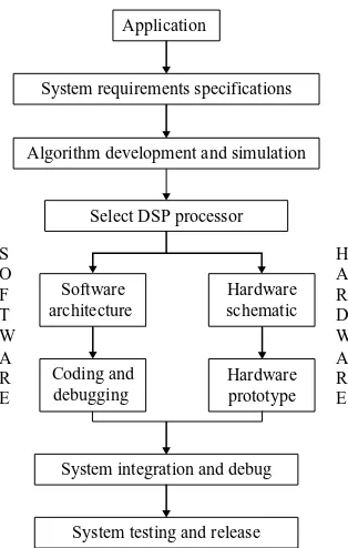
1.4 DSP System Design 17
1.4.1 Algorithm Development 18
1.4.2 Selection of DSP Processors 19
1.4.3 Software Development 20
1.4.4 High-Level Software Development Tools 21
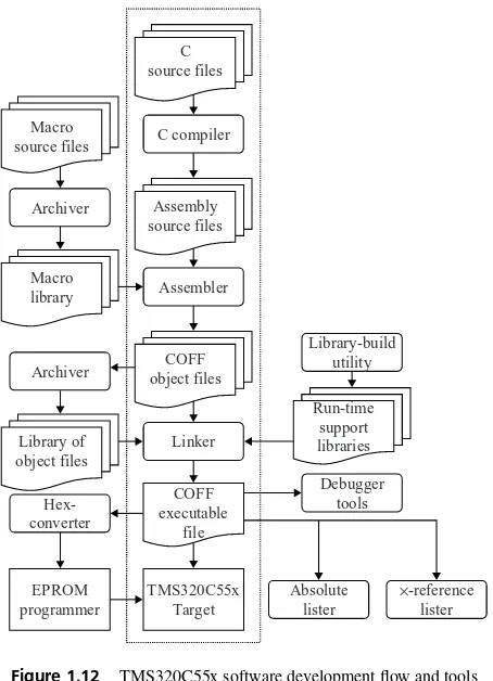
1.5 Introduction to DSP Development Tools 22
1.5.1 C Compiler 22
1.5.2 Assembler 23
1.5.3 Linker 24
1.5.4 Other Development Tools 25
1.6 Experiments and Program Examples 25
1.6.1 Experiments of Using CCS and DSK 26
1.6.2 Debugging Program Using CCS and DSK 29
1.6.3 File I/O Using Probe Point 32
1.6.4 File I/O Using C File System Functions 35
1.6.5 Code Efficiency Analysis Using Profiler 37
1.6.6 Real-Time Experiments Using DSK 39
1.6.7 Sampling Theory 42
1.6.8 Quantization in ADCs 44
References 45
2 Introduction to TMS320C55x Digital Signal Processor
49
2.2.5 Interrupts and Interrupt Vector 55
2.3 TMS320C55x Peripherals 58
2.3.1 External Memory Interface 60
2.3.2 Direct Memory Access 60
2.3.3 Enhanced Host-Port Interface 61
2.3.4 Multi-Channel Buffered Serial Ports 62
2.3.5 Clock Generator and Timers 65
2.3.6 General Purpose Input/Output Port 65
2.4 TMS320C55x Addressing Modes 65
2.4.1 Direct Addressing Modes 66
2.4.2 Indirect Addressing Modes 68
2.4.3 Absolute Addressing Modes 70
2.4.4 Memory-Mapped Register Addressing Mode 70
2.4.5 Register Bits Addressing Mode 71
2.4.6 Circular Addressing Mode 72
2.5 Pipeline and Parallelism 73
2.5.1 TMS320C55x Pipeline 73
2.5.2 Parallel Execution 74
2.6 TMS320C55x Instruction Set 76
2.6.1 Arithmetic Instructions 76
2.6.2 Logic and Bit Manipulation Instructions 77
2.6.3 Move Instruction 78
2.6.4 Program Flow Control Instructions 78
2.7 TMS320C55x Assembly Language Programming 82
2.7.1 Assembly Directives 82
2.7.2 Assembly Statement Syntax 84
2.8 C Language Programming for TMS320C55x 86
2.8.1 Data Types 86
2.8.2 Assembly Code Generation by C Compiler 87
2.8.3 Compiler Keywords and Pragma Directives 89
2.9 Mixed C-and-Assembly Language Programming 90
2.10 Experiments and Program Examples 93
2.10.1 Interfacing C with Assembly Code 93
2.10.2 Addressing Modes Using Assembly Programming 94
2.10.3 Phase-Locked Loop and Timers 97
2.10.4 EMIF Configuration for Using SDRAM 103
2.10.5 Programming Flash Memory Devices 105
2.10.6 Using McBSP 106
2.10.7 AIC23 Configurations 109
2.10.8 Direct Memory Access 111
References 115
3 DSP Fundamentals and Implementation
Considerations
121
3.1 Digital Signals and Systems 121
3.1.1 Elementary Digital Signals 121
3.1.2 Block Diagram Representation of Digital Systems 123
3.2 System Concepts 126
3.2.1 Linear Time-Invariant Systems 126
3.2.2 Thez-Transform 130
3.2.3 Transfer Functions 132
3.2.4 Poles and Zeros 135
3.2.5 Frequency Responses 138
3.2.6 Discrete Fourier Transform 141
3.3 Introduction to Random Variables 142
3.3.1 Review of Random Variables 142
3.3.2 Operations of Random Variables 144
3.4 Fixed-Point Representations and Quantization Effects 147
3.4.1 Fixed-Point Formats 147
3.4.2 Quantization Errors 151
3.4.3 Signal Quantization 151
3.4.4 Coefficient Quantization 153
3.4.5 Roundoff Noise 153
3.4.6 Fixed-Point Toolbox 154
3.5 Overflow and Solutions 157
3.5.1 Saturation Arithmetic 157
3.5.2 Overflow Handling 158
3.5.3 Scaling of Signals 158
3.5.4 Guard Bits 159
3.6 Experiments and Program Examples 159
3.6.1 Quantization of Sinusoidal Signals 160
3.6.2 Quantization of Audio Signals 161
3.6.3 Quantization of Coefficients 162
3.6.4 Overflow and Saturation Arithmetic 164
3.6.5 Function Approximations 167
3.6.6 Real-Time Digital Signal Generation Using DSK 175
References 180
Exercises 180
4 Design and Implementation of FIR Filters
185
4.1 Introduction to FIR Filters 185
4.1.1 Filter Characteristics 185
4.1.2 Filter Types 187
4.1.3 Filter Specifications 189
4.1.4 Linear-Phase FIR Filters 191
4.1.5 Realization of FIR Filters 194
4.2 Design of FIR Filters 196
4.2.1 Fourier Series Method 197
4.2.2 Gibbs Phenomenon 198
4.2.4 Design of FIR Filters Using MATLAB 206
4.2.5 Design of FIR Filters Using FDATool 207
4.3 Implementation Considerations 213
4.3.1 Quantization Effects in FIR Filters 213
4.3.2 MATLAB Implementations 216
4.3.3 Floating-Point C Implementations 218
4.3.4 Fixed-Point C Implementations 219
4.4 Applications: Interpolation and Decimation Filters 220
4.4.1 Interpolation 220
4.4.2 Decimation 221
4.4.3 Sampling-Rate Conversion 221
4.4.4 MATLAB Implementations 224
4.5 Experiments and Program Examples 225
4.5.1 Implementation of FIR Filters Using Fixed-Point C 226 4.5.2 Implementation of FIR Filter Using C55x Assembly
Language 226
4.5.3 Optimization for Symmetric FIR Filters 228
4.5.4 Optimization Using Dual MAC Architecture 230
4.5.5 Implementation of Decimation 232
4.5.6 Implementation of Interpolation 233
4.5.7 Sample Rate Conversion 234
4.5.8 Real-Time Sample Rate Conversion Using
DSP/BIOS and DSK 235
References 245
Exercises 245
5 Design and Implementation of IIR Filters
249
5.1 Introduction 249
5.1.1 Analog Systems 249
5.1.2 Mapping Properties 251
5.1.3 Characteristics of Analog Filters 252
5.1.4 Frequency Transforms 254
5.2 Design of IIR Filters 255
5.2.1 Bilinear Transform 256
5.2.2 Filter Design Using Bilinear Transform 257
5.3 Realization of IIR Filters 258
5.3.1 Direct Forms 258
5.3.2 Cascade Forms 260
5.3.3 Parallel Forms 262
5.3.4 Realization of IIR Filters Using MATLAB 263
5.4 Design of IIR Filters Using MATLAB 264
5.4.1 Filter Design Using MATLAB 264
5.4.2 Frequency Transforms Using MATLAB 267
5.4.3 Design and Realization Using FDATool 268
5.5 Implementation Considerations 271
5.5.1 Stability 271
5.5.2 Finite-Precision Effects and Solutions 273
5.6 Practical Applications 279
5.6.1 Recursive Resonators 279
5.6.2 Recursive Quadrature Oscillators 282
5.6.3 Parametric Equalizers 284
5.7 Experiments and Program Examples 285
5.7.1 Floating-Point Direct-Form I IIR Filter 285
5.7.2 Fixed-Point Direct-Form I IIR Filter 286
5.7.3 Fixed-Point Direct-Form II Cascade IIR Filter 287
5.7.4 Implementation Using DSP Intrinsics 289
5.7.5 Implementation Using Assembly Language 290
5.7.6 Real-Time Experiments Using DSP/BIOS 293
5.7.7 Implementation of Parametric Equalizer 296
5.7.8 Real-Time Two-Band Equalizer Using DSP/BIOS 297
References 299
Exercises 299
6 Frequency Analysis and Fast Fourier Transform
303
6.1 Fourier Series and Transform 303
6.1.1 Fourier Series 303
6.1.2 Fourier Transform 304
6.2 Discrete Fourier Transform 305
6.2.1 Discrete-Time Fourier Transform 305
6.2.2 Discrete Fourier Transform 307
6.2.3 Important Properties 310
6.3 Fast Fourier Transforms 313
6.3.1 Decimation-in-Time 314
6.3.2 Decimation-in-Frequency 316
6.3.3 Inverse Fast Fourier Transform 317
6.4 Implementation Considerations 317
6.4.1 Computational Issues 317
6.4.2 Finite-Precision Effects 318
6.4.3 MATLAB Implementations 318
6.4.4 Fixed-Point Implementation Using MATLAB 320
6.5 Practical Applications 322
6.5.1 Spectral Analysis 322
6.5.2 Spectral Leakage and Resolution 323
6.5.3 Power Spectrum Density 325
6.5.4 Fast Convolution 328
6.6 Experiments and Program Examples 332
6.6.1 Floating-Point C Implementation of DFT 332
6.6.2 C55x Assembly Implementation of DFT 332
6.6.3 Floating-Point C Implementation of FFT 336
6.6.4 C55x Intrinsics Implementation of FFT 338
6.6.5 Assembly Implementation of FFT and Inverse FFT 339
6.6.6 Implementation of Fast Convolution 343
6.6.7 Real-Time FFT Using DSP/BIOS 345
6.6.8 Real-Time Fast Convolution 347
References 347
7 Adaptive Filtering
351
7.1 Introduction to Random Processes 351
7.2 Adaptive Filters 354
7.2.1 Introduction to Adaptive Filtering 354
7.2.2 Performance Function 355
7.2.3 Method of Steepest Descent 358
7.2.4 The LMS Algorithm 360
7.2.5 Modified LMS Algorithms 361
7.3 Performance Analysis 362
7.3.1 Stability Constraint 362
7.3.2 Convergence Speed 363
7.3.3 Excess Mean-Square Error 363
7.3.4 Normalized LMS Algorithm 364
7.4 Implementation Considerations 364
7.4.1 Computational Issues 365
7.4.2 Finite-Precision Effects 365
7.4.3 MATLAB Implementations 366
7.5 Practical Applications 368
7.5.1 Adaptive System Identification 368
7.5.2 Adaptive Linear Prediction 369
7.5.3 Adaptive Noise Cancelation 372
7.5.4 Adaptive Notch Filters 374
7.5.5 Adaptive Channel Equalization 375
7.6 Experiments and Program Examples 377
7.6.1 Floating-Point C Implementation 377
7.6.2 Fixed-Point C Implementation of Leaky LMS Algorithm 379
7.6.3 ETSI Implementation of NLMS Algorithm 380
7.6.4 Assembly Language Implementation of Delayed LMS Algorithm 383
7.6.5 Adaptive System Identification 387
7.6.6 Adaptive Prediction and Noise Cancelation 388
7.6.7 Adaptive Channel Equalizer 392
7.6.8 Real-Time Adaptive Line Enhancer Using DSK 394
References 396
Exercises 397
8 Digital Signal Generators
401
8.1 Sinewave Generators 401
8.1.1 Lookup-Table Method 401
8.1.2 Linear Chirp Signal 404
8.2 Noise Generators 405
8.2.1 Linear Congruential Sequence Generator 405
8.2.2 Pseudo-Random Binary Sequence Generator 407
8.3 Practical Applications 409
8.3.1 Siren Generators 409
8.3.2 White Gaussian Noise 409
8.3.3 Dual-Tone Multifrequency Tone Generator 410
8.3.4 Comfort Noise in Voice Communication Systems 411
8.4 Experiments and Program Examples 412
8.4.1 Sinewave Generator Using C5510 DSK 412
8.4.3 Wail Siren Generator Using C5510 DSK 414
8.4.4 DTMF Generator Using C5510 DSK 415
8.4.5 DTMF Generator Using MATLAB Graphical User Interface 416
References 418
Exercises 418
9 Dual-Tone Multifrequency Detection
421
9.1 Introduction 421
9.2 DTMF Tone Detection 422
9.2.1 DTMF Decode Specifications 422
9.2.2 Goertzel Algorithm 423
9.2.3 Other DTMF Detection Methods 426
9.2.4 Implementation Considerations 428
9.3 Internet Application Issues and Solutions 431
9.4 Experiments and Program Examples 432
9.4.1 Implementation of Goertzel Algorithm Using Fixed-Point C 432 9.4.2 Implementation of Goertzel Algorithm Using C55x
Assembly Language 434
9.4.3 DTMF Detection Using C5510 DSK 435
9.4.4 DTMF Detection Using All-Pole Modeling 439
References 441
Exercises 442
10 Adaptive Echo Cancelation
443
10.1 Introduction to Line Echoes 443
10.2 Adaptive Echo Canceler 444
10.2.1 Principles of Adaptive Echo Cancelation 445
10.2.2 Performance Evaluation 446
10.3 Practical Considerations 447
10.3.1 Prewhitening of Signals 447
10.3.2 Delay Detection 448
10.4 Double-Talk Effects and Solutions 450
10.5 Nonlinear Processor 453
10.5.1 Center Clipper 453
10.5.2 Comfort Noise 453
10.6 Acoustic Echo Cancelation 454
10.6.1 Acoustic Echoes 454
10.6.2 Acoustic Echo Canceler 456
10.6.3 Subband Implementations 457
10.6.4 Delay-Free Structures 459
10.6.5 Implementation Considerations 459
10.6.6 Testing Standards 460
10.7 Experiments and Program Examples 461
10.7.1 MATLAB Implementation of AEC 461
10.7.2 Acoustic Echo Cancelation Using Floating-Point C 464
10.7.3 Acoustic Echo Canceler Using C55x Intrinsics 468
10.7.4 Experiment of Delay Estimation 469
References 472
11 Speech-Coding Techniques
475
11.1 Introduction to Speech-Coding 475
11.2 Overview of CELP Vocoders 476
11.2.1 Synthesis Filter 477
11.2.2 Long-Term Prediction Filter 481
11.2.3 Perceptual Based Minimization Procedure 481
11.2.4 Excitation Signal 482
11.2.5 Algebraic CELP 483
11.3 Overview of Some Popular CODECs 484
11.3.1 Overview of G.723.1 484
11.3.2 Overview of G.729 488
11.3.3 Overview of GSM AMR 490
11.4 Voice over Internet Protocol Applications 492
11.4.1 Overview of VoIP 492
11.4.2 Real-Time Transport Protocol and Payload Type 493
11.4.3 Example of Packing G.729 496
11.4.4 RTP Data Analysis Using Ethereal Trace 496
11.4.5 Factors Affecting the Overall Voice Quality 497
11.5 Experiments and Program Examples 497
11.5.1 Calculating LPC Coefficients Using Floating-Point C 497 11.5.2 Calculating LPC Coefficients Using C55x Intrinsics 499 11.5.3 MATLAB Implementation of Formant Perceptual Weighting Filter 504 11.5.4 Implementation of Perceptual Weighting Filter Using C55x Intrinsics 506
References 507
Exercises 508
12 Speech Enhancement Techniques
509
12.1 Introduction to Noise Reduction Techniques 509
12.2 Spectral Subtraction Techniques 510
12.2.1 Short-Time Spectrum Estimation 511
12.2.2 Magnitude Subtraction 511
12.3 Voice Activity Detection 513
12.4 Implementation Considerations 515
12.4.1 Spectral Averaging 515
12.4.2 Half-Wave Rectification 515
12.4.3 Residual Noise Reduction 516
12.5 Combination of Acoustic Echo Cancelation with NR 516
12.6 Voice Enhancement and Automatic Level Control 518
12.6.1 Voice Enhancement Devices 518
12.6.2 Automatic Level Control 519
12.7 Experiments and Program Examples 519
12.7.1 Voice Activity Detection 519
12.7.2 MATLAB Implementation of NR Algorithm 522
12.7.3 Floating-Point C Implementation of NR 522
12.7.4 Mixed C55x Assembly and Intrinsics Implementations of VAD 522
12.7.5 Combining AEC with NR 526
References 529
13 Audio Signal Processing
531
13.1 Introduction 531
13.2 Basic Principles of Audio Coding 531
13.2.1 Auditory-Masking Effects for Perceptual Coding 533
13.2.2 Frequency-Domain Coding 536
13.2.3 Lossless Audio Coding 538
13.3 Multichannel Audio Coding 539
13.3.1 MP3 540
13.3.2 Dolby AC-3 541
13.3.3 MPEG-2 AAC 542
13.4 Connectivity Processing 544
13.5 Experiments and Program Examples 544
13.5.1 Floating-Point Implementation of MDCT 544
13.5.2 Implementation of MDCT Using C55x Intrinsics 547
13.5.3 Experiments of Preecho Effects 549
13.5.4 Floating-Point C Implementation of MP3 Decoding 549
References 553
Exercises 553
14 Channel Coding Techniques
555
14.1 Introduction 555
14.2 Block Codes 556
14.2.1 Reed–Solomon Codes 558
14.2.2 Applications of Reed–Solomon Codes 562
14.2.3 Cyclic Redundant Codes 563
14.3 Convolutional Codes 564
14.3.1 Convolutional Encoding 564
14.3.2 Viterbi Decoding 564
14.3.3 Applications of Viterbi Decoding 566
14.4 Experiments and Program Examples 569
14.4.1 Reed–Solomon Coding Using MATALB 569
14.4.2 Reed–Solomon Coding Using Simulink 570
14.4.3 Verification of RS(255, 239) Generation Polynomial 571
14.4.4 Convolutional Codes 572
14.4.5 Implementation of Convolutional Codes Using C 573
14.4.6 Implementation of CRC-32 575
References 576
Exercises 577
15 Introduction to Digital Image Processing
579
15.1 Digital Images and Systems 579
15.1.1 Digital Images 579
15.1.2 Digital Image Systems 580
15.2 RGB Color Spaces and Color Filter Array Interpolation 581
15.3 Color Spaces 584
15.3.1 YCbCrand YUV Color Spaces 584
15.3.3 YIQ Color Space 585
15.3.4 HSV Color Space 585
15.4 YCbCrSubsampled Color Spaces 586
15.5 Color Balance and Correction 586
15.5.1 Color Balance 587
15.5.2 Color Adjustment 588
15.5.3 Gamma Correction 589
15.6 Image Histogram 590
15.7 Image Filtering 591
15.8 Image Filtering Using Fast Convolution 596
15.9 Practical Applications 597
15.9.1 JPEG Standard 597
15.9.2 2-D Discrete Cosine Transform 599
15.10 Experiments and Program Examples 601
15.10.1 YCbCrto RGB Conversion 601
15.10.2 Using CCS Link with DSK and Simulator 604
15.10.3 White Balance 607
15.10.4 Gamma Correction and Contrast Adjustment 610
15.10.5 Histogram and Histogram Equalization 611
15.10.6 2-D Image Filtering 613
15.10.7 Implementation of DCT and IDCT 617
15.10.8 TMS320C55x Image Accelerator for DCT and IDCT 621
15.10.9 TMS320C55x Hardware Accelerator Image/Video Processing Library 623
References 625
Exercises 625
Appendix A Some Useful Formulas and Definitions
627
A.1 Trigonometric Identities 627
A.2 Geometric Series 628
A.3 Complex Variables 628
A.4 Units of Power 630
References 631
Appendix B Software Organization and List of Experiments
633
Preface
In recent years, digital signal processing (DSP) has expanded beyond filtering, frequency analysis, and signal generation. More and more markets are opening up to DSP applications, where in the past, real-time signal processing was not feasible or was too expensive. Real-time signal processing using general-purpose DSP processors provides an effective way to design and implement DSP algorithms for real-world applications. However, this is very challenging work in today’s engineering fields. With DSP penetrating into many practical applications, the demand for high-performance digital signal processors has expanded rapidly in recent years. Many industrial companies are currently engaged in real-time DSP research and development. Therefore, it becomes increasingly important for today’s students, practicing engineers, and development researchers to master not only the theory of DSP, but also the skill of real-time DSP system design and implementation techniques.
This book provides fundamental real-time DSP principles and uses a hands-on approach to introduce DSP algorithms, system design, real-time implementation considerations, and many practical applica-tions. This book contains many useful examples like hands-on experiment software and DSP programs using MATLAB, Simulink, C, and DSP assembly languages. Also included are various exercises for further exploring the extensions of the examples and experiments. The book uses the Texas Instruments’ Code Composer Studio (CCS) with the Spectrum Digital TMS320VC5510 DSP starter kit (DSK) devel-opment tool for real-time experiments and applications.
This book emphasizes real-time DSP applications and is intended as a text for senior/graduate-level college students. The prerequisites of this book are signals and systems concepts, microprocessor ar-chitecture and programming, and basic C programming knowledge. These topics are covered at the sophomore and junior levels of electrical and computer engineering, computer science, and other related engineering curricula. This book can also serve as a desktop reference for DSP engineers, algorithm developers, and embedded system programmers to learn DSP concepts and to develop real-time DSP applications on the job. We use a practical approach that avoids numerous theoretical derivations. A list of DSP textbooks with mathematical proofs is given at the end of each chapter. Also helpful are the manuals and application notes for the TMS320C55x DSP processors from Texas Instruments atwww.ti.com, and for the MATLAB and Simulink from Math Works atwww.mathworks.com.
This is the second edition of the book titled ‘Real-Time Digital Signal Processing: Implementations, Applications and Experiments with the TMS320C55x’ by Kuo and Lee, John Wiley & Sons, Ltd. in 2001. The major changes included in the revision are:
on fixed-point DSP processors. This step-by-step software development and optimization process is applied to the finite-impulse response (FIR) filtering, infinite-impulse response (IIR) filtering, adaptive filtering, fast Fourier transform, and many real-life applications in Chapters 8–15. 2. To add several widely used DSP applications such as speech coding, channel coding, audio coding,
image processing, signal generation and detection, echo cancelation, and noise reduction by expand-ing Chapter 9 of the first edition to eight new chapters with the necessary background to perform the experiments using the optimized software development process.
3. To design and analyze DSP algorithms using the most effective MATLAB graphic user interface (GUI) tools such as Signal Processing Tool (SPTool), Filter Design and Analysis Tool (FDATool), etc. These tools are powerful for filter designing, analysis, quantization, testing, and implementation. 4. To add step-by-step experiments to create CCS DSP/BIOS applications, configure the TMS320VC5510 DSK for real-time audio applications, and utilize MATLAB’s Link for CCS feature to improve DSP development, debug, analyze, and test efficiencies.
5. To update experiments to include new sets of hands-on exercises and applications. Also, to update all programs using the most recent version of software and the TMS320C5510 DSK board for real-time experiments.
There are many existing DSP algorithms and applications available in MATLAB and floating-point C programs. This book provides a systematic software development process for converting these pro-grams to fixed-point C and optimizing them for implementation on commercially available fixed-point DSP processors. To effectively illustrate real-time DSP concepts and applications, MATLAB is used for analysis and filter design, C program is used for implementing DSP algorithms, and CCS is in-tegrated into TMS320C55x experiments and applications. To efficiently utilize the advanced DSP ar-chitecture for fast software development and maintenance, the mixing of C and assembly programs is emphasized.
This book is organized into two parts: DSP implementation and DSP application. Part I, DSP implemen-tation (Chapters 1–7) discusses real-time DSP principles, architectures, algorithms, and implemenimplemen-tation considerations. Chapter 1 reviews the fundamentals of real-time DSP functional blocks, DSP hardware options, fixed- and floating-point DSP devices, real-time constraints, algorithm development, selection of DSP chips, and software development. Chapter 2 introduces the architecture and assembly programming of the TMS320C55x DSP processor. Chapter 3 presents fundamental DSP concepts and practical con-siderations for the implementation of digital filters and algorithms on DSP hardware. Chapter 4 focuses on the design, implementation, and application of FIR filters. Digital IIR filters are covered in Chapter 5, and adaptive filters are presented in Chapter 7. The development, implementation, and application of FFT algorithms are introduced in Chapter 6.
Part II, DSP application (Chapters 8–15) introduces several popular real-world applications in signal processing that have played important roles in the realization of the systems. These selected DSP applica-tions include signal (sinewave, noise, and multitone) generation in Chapter 8, dual-tone multifrequency detection in Chapter 9, adaptive echo cancelation in Chapter 10, speech-coding algorithms in Chapter 11, speech enhancement techniques in Chapter 12, audio coding methods in Chapter 13, error correction coding techniques in Chapter 14, and image processing fundamentals in Chapter 15.
Software Availability
This text utilizes various MATLAB, floating-point and fixed-point C, DSP assembly and mixed C and assembly programs for the examples, experiments, and applications. These programs along with many other programs and real-world data files are available in the companion CD. The directory structure and the subdirectory names are explained in Appendix B. The software will assist in gaining insight into the understanding and implementation of DSP algorithms, and it is required for doing experiments in the last section of each chapter. Some of these experiments involve minor modifications of the example code. By examining, studying, and modifying the example code, the software can also be used as a prototype for other practical applications. Every attempt has been made to ensure the correctness of the code. We would appreciate readers bringing to our attention ([email protected]) any coding errors so that we can correct, update, and post them on the websitehttp://www.ceet.niu.edu/faculty/kuo.
Acknowledgments
We are grateful to Cathy Wicks and Gene Frantz of Texas Instruments, and to Naomi Fernandes and Courtney Esposito of The MathWorks for providing us with the support needed to write this book. We would like to thank several individuals at Wiley for their support on this project: Simone Taylor, Executive Commissioning Editor; Emily Bone, Assistant Editor; and Lucy Bryan, Executive Project Editor. We also thank the staff at Wiley for the final preparation of this book. Finally, we thank our families for the endless love, encouragement, patience, and understanding they have shown throughout this period.
1
Introduction to Real-Time
Digital Signal Processing
Signals can be divided into three categories: continuous-time (analog) signals, discrete-time signals, and digital signals. The signals that we encounter daily are mostly analog signals. These signals are defined continuously in time, have an infinite range of amplitude values, and can be processed using analog electronics containing both active and passive circuit elements. Discrete-time signals are defined only at a particular set of time instances. Therefore, they can be represented as a sequence of numbers that have a continuous range of values. Digital signals have discrete values in both time and amplitude; thus, they can be processed by computers or microprocessors. In this book, we will present the design, implementation, and applications of digital systems for processing digital signals using digital hardware. However, the analysis usually uses discrete-time signals and systems for mathematical convenience. Therefore, we use the terms ‘discrete-time’ and ‘digital’ interchangeably.
Digital signal processing (DSP) is concerned with the digital representation of signals and the use of digital systems to analyze, modify, store, or extract information from these signals. Much research has been conducted to develop DSP algorithms and systems for real-world applications. In recent years, the rapid advancement in digital technologies has supported the implementation of sophisti-cated DSP algorithms for real-time applications. DSP is now used not only in areas where analog methods were used previously, but also in areas where applying analog techniques is very difficult or impossible.
There are many advantages in using digital techniques for signal processing rather than traditional analog devices, such as amplifiers, modulators, and filters. Some of the advantages of a DSP system over analog circuitry are summarized as follows:
1. Flexibility: Functions of a DSP system can be easily modified and upgraded with software that implements the specific applications. One can design a DSP system that can be programmed to perform a wide variety of tasks by executing different software modules. A digital electronic device can be easily upgraded in the field through the onboard memory devices (e.g., flash memory) to meet new requirements or improve its features.
2. Reproducibility: The performance of a DSP system can be repeated precisely from one unit to another. In addition, by using DSP techniques, digital signals such as audio and video streams can be stored, transferred, or reproduced many times without degrading the quality. By contract, analog circuits
Real-Time Digital Signal Processing: Implementations and Applications S.M. Kuo, B.H. Lee, and W. Tian C
will not have the same characteristics even if they are built following identical specifications due to analog component tolerances.
3. Reliability: The memory and logic of DSP hardware does not deteriorate with age. Therefore, the field performance of DSP systems will not drift with changing environmental conditions or aged electronic components as their analog counterparts do.
4. Complexity: DSP allows sophisticated applications such as speech recognition and image compres-sion to be implemented with lightweight and low-power portable devices. Furthermore, there are some important signal processing algorithms such as error correcting codes, data transmission and storage, and data compression, which can only be performed using DSP systems.
With the rapid evolution in semiconductor technologies, DSP systems have a lower overall cost com-pared to analog systems for most applications. DSP algorithms can be developed, analyzed, and simulated using high-level language and software tools such as C/C++and MATLAB (matrix laboratory). The performance of the algorithms can be verified using a low-cost, general-purpose computer. Therefore, a DSP system is relatively easy to design, develop, analyze, simulate, test, and maintain.
There are some limitations associated with DSP. For instance, the bandwidth of a DSP system is limited by the sampling rate and hardware peripherals. Also, DSP algorithms are implemented using a fixed number of bits with a limited precision and dynamic range (the ratio between the largest and smallest numbers that can be represented), which results in quantization and arithmetic errors. Thus, the system performance might be different from the theoretical expectation.
1.1 Basic Elements of Real-Time DSP Systems
There are two types of DSP applications: non-real-time and real-time. Non-real-time signal processing involves manipulating signals that have already been collected in digital forms. This may or may not represent a current action, and the requirement for the processing result is not a function of real time. Real-time signal processing places stringent demands on DSP hardware and software designs to complete predefined tasks within a certain time frame. This chapter reviews the fundamental functional blocks of real-time DSP systems.
The basic functional blocks of DSP systems are illustrated in Figure 1.1, where a real-world analog signal is converted to a digital signal, processed by DSP hardware, and converted back into an analog
Other digital
signal. Each of the functional blocks in Figure 1.1 will be introduced in the subsequent sections. For some applications, the input signal may already be in digital form and/or the output data may not need to be converted to an analog signal. For example, the processed digital information may be stored in computer memory for later use, or it may be displayed graphically. In other applications, the DSP system may be required to generate signals digitally, such as speech synthesis used for computerized services or pseudo-random number generators for CDMA (code division multiple access) wireless communication systems.
1.2 Analog Interface
In this book, a time-domain signal is denoted with a lowercase letter. For example,x(t) in Figure 1.1 is used to name an analog signal ofxwhich is a function of timet. The time variabletand the amplitude of x(t) take on a continuum of values between−∞and∞. For this reason we sayx(t) is a continuous-time signal. The signalsx(n) andy(n) in Figure 1.1 depict digital signals which are only meaningful at time instantn. In this section, we first discuss how to convert analog signals into digital signals so that they can be processed using DSP hardware. The process of converting an analog signal to a digital signal is called the analog-to-digital conversion, usually performed by an analog-to-digital converter (ADC).
The purpose of signal conversion is to prepare real-world analog signals for processing by digital hardware. As shown in Figure 1.1, the analog signalx′(t) is picked up by an appropriate electronic sensor that converts pressure, temperature, or sound into electrical signals. For example, a microphone can be used to collect sound signals. The sensor signalx′(t) is amplified by an amplifier with gain valueg. The amplified signal is
x(t)=gx′(t). (1.1)
The gain valuegis determined such thatx(t) has a dynamic range that matches the ADC used by the system. If the peak-to-peak voltage range of the ADC is±5 V, thengmay be set so that the amplitude of signalx(t) to the ADC is within±5 V. In practice, it is very difficult to set an appropriate fixed gain because the level ofx′(t) may be unknown and changing with time, especially for signals with a larger dynamic range such as human speech.
Once the input digital signal has been processed by the DSP hardware, the resulty(n) is still in digital form. In many DSP applications, we need to reconstruct the analog signal after the completion of digital processing. We must convert the digital signaly(n) back to the analog signaly(t) before it is applied to an appropriated analog device. This process is called the digital-to-analog conversion, typically performed by a digital-to-analog converter (DAC). One example would be audio CD (compact disc) players, for which the audio music signals are stored in digital form on CDs. A CD player reads the encoded digital audio signals from the disk and reconstructs the corresponding analog waveform for playback via loudspeakers. The system shown in Figure 1.1 is a real-time system if the signal to the ADC is continuously sampled and the ADC presents a new sample to the DSP hardware at the same rate. In order to maintain real-time operation, the DSP hardware must perform all required operations within the fixed time period, and present an output sample to the DAC before the arrival of the next sample from the ADC.
1.2.1 Sampling
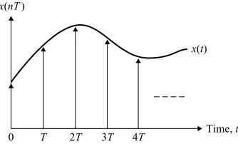
x(t)
Ideal sampler
x(nT)
Quantizer
x(n) Analog-to-digital converter
Figure 1.2 Block diagram of an ADC
Quantization process approximates a waveform by assigning a number for each sample. Therefore, the analog-to-digital conversion will perform the following steps:
1. The bandlimited signalx(t) is sampled at uniformly spaced instants of timenT, wherenis a positive integer andT is the sampling period in seconds. This sampling process converts an analog signal into a discrete-time signalx(nT) with continuous amplitude value.
2. The amplitude of each discrete-time sample is quantized into one of the 2B levels, whereBis the number of bits that the ADC has to represent for each sample. The discrete amplitude levels are represented (or encoded) into distinct binary wordsx(n) with a fixed wordlengthB.
The reason for making this distinction is that these processes introduce different distortions. The sampling process brings in aliasing or folding distortion, while the encoding process results in quantization noise. As shown in Figure 1.2, the sampler and quantizer are integrated on the same chip. However, high-speed ADCs typically require an external sample-and-hold device.
An ideal sampler can be considered as a switch that periodically opens and closes everyTs (seconds). The sampling period is defined as
T = 1 fs
, (1.2)
where fsis the sampling frequency (or sampling rate) in hertz (or cycles per second). The intermediate signalx(nT) is a discrete-time signal with a continuous value (a number with infinite precision) at discrete timenT,n=0, 1, . . . ,∞, as illustrated in Figure 1.3. The analog signalx(t) is continuous in both time and amplitude. The sampled discrete-time signalx(nT) is continuous in amplitude, but is defined only at discrete sampling instantst=nT.
Time, t x(nT)
0 T 2T 3T 4T
x(t)
In order to represent an analog signalx(t) by a discrete-time signalx(nT) accurately, the sampling frequency fsmust be at least twice the maximum frequency component (fM) in the analog signalx(t). That is,
fs≥2fM, (1.3)
wherefMis also called the bandwidth of the signalx(t). This is Shannon’s sampling theorem, which states that when the sampling frequency is greater than twice of the highest frequency component contained in the analog signal, the original signalx(t) can be perfectly reconstructed from the corresponding discrete-time signalx(nT).
The minimum sampling rate fs=2fMis called the Nyquist rate. The frequency fN= fs/2 is called the Nyquist frequency or folding frequency. The frequency interval [−fs/2, fs/2] is called the Nyquist interval. When an analog signal is sampled at fs, frequency components higher than fs/2 fold back into the frequency range [0, fs/2]. The folded back frequency components overlap with the original frequency components in the same range. Therefore, the original analog signal cannot be recovered from the sampled data. This undesired effect is known as aliasing.
Example 1.1:Consider two sinewaves of frequencies f1=1 Hz and f2=5 Hz that are sampled at fs=4 Hz, rather than at 10 Hz according to the sampling theorem. The analog waveforms are illustrated in Figure 1.4(a), while their digital samples and reconstructed waveforms are illustrated
x(t), f1= 1Hz x(t), f2= 5Hz
t, second
x(t)
x(n)
t
x(n) x(t)
(a) Original analog waveforms and digital samplses for f1 = 1 Hz and f2 = 5 Hz.
x(n), f1= 1Hz x(n), f2= 5Hz
n x(t)
x(n)
x(n)
x(t)
n
(b) Digital samples for f1 = 1 Hz and f2 = 5 Hz and reconstructed waveforms.
in Figure 1.4(b). As shown in the figures, we can reconstruct the original waveform from the digital samples for the sinewave of frequency f1=1 Hz. However, for the original sinewave of frequency f2=5 Hz, the reconstructed signal is identical to the sinewave of frequency 1 Hz. Therefore, f1 and f2are said to be aliased to one another, i.e., they cannot be distinguished by their discrete-time samples.
Note that the sampling theorem assumes that the signal is bandlimited. For most practical applications, the analog signalx(t) may have significant energies outside the highest frequency of interest, or may contain noise with a wider bandwidth. In some cases, the sampling rate is predetermined by a given application. For example, most voice communication systems use an 8 kHz sampling rate. Unfortunately, the frequency components in a speech signal can be much higher than 4 kHz. To guarantee that the sampling theorem defined in Equation (1.3) can be fulfilled, we must block the frequency components that are above the Nyquist frequency. This can be done by using an antialiasing filter, which is an analog lowpass filter with the cutoff frequency
fc≤ fs
2. (1.4)
Ideally, an antialiasing filter should remove all frequency components above the Nyquist frequency. In many practical systems, a bandpass filter is preferred to remove all frequency components above the Nyquist frequency, as well as to prevent undesired DC offset, 60 Hz hum, or other low-frequency noises. A bandpass filter with passband from 300 to 3200 Hz can often be found in telecommunication systems. Since antialiasing filters used in real-world applications are not ideal filters, they cannot completely remove all frequency components outside the Nyquist interval. In addition, since the phase response of the analog filter may not be linear, the phase of the signal will not be shifted by amounts proportional to their frequencies. In general, a lowpass (or bandpass) filter with steeper roll-off will introduce more phase distortion. Higher sampling rates allow simple low-cost antialiasing filter with minimum phase distortion to be used. This technique is known as oversampling, which is widely used in audio applications.
Example 1.2:The range of sampling rate required by DSP systems is large, from approximately 1 GHz in radar to 1 Hz in instrumentation. Given a sampling rate for a specific application, the sampling period can be determined by (1.2). Some real-world applications use the following sampling frequencies and periods:
1. In International Telecommunication Union (ITU) speech compression standards, the sampling rate of ITU-T G.729 and G.723.1 is fs=8 kHz, thus the sampling periodT =1/8000 s= 125μs. Note that 1μs=10−6s.
2. Wideband telecommunication systems, such as ITU-T G.722, use a sampling rate of fs = 16 kHz, thusT =1/16 000 s=62.5μs.
3. In audio CDs, the sampling rate is fs=44.1 kHz, thusT =1/44 100 s=22.676μs. 4. High-fidelity audio systems, such as MPEG-2 (moving picture experts group) AAC (advanced
audio coding) standard, MP3 (MPEG layer 3) audio compression standard, and Dolby AC-3, have a sampling rate of fs =48 kHz, and thusT =1/48 000 s=20.833μs. The sampling rate for MPEG-2 AAC can be as high as 96 kHz.
1.2.2 Quantization and Encoding
In previous sections, we assumed that the sample valuesx(nT) are represented exactly with an infinite number of bits (i.e.,B→ ∞). We now discuss a method of representing the sampled discrete-time signal x(nT) as a binary number with finite number of bits. This is the quantization and encoding process. If the wordlength of an ADC isBbits, there are 2B different values (levels) that can be used to represent a sample. Ifx(n) lies between two quantization levels, it will be either rounded or truncated. Rounding replacesx(n) by the value of the nearest quantization level, while truncation replacesx(n) by the value of the level below it. Since rounding produces less biased representation of the analog values, it is widely used by ADCs. Therefore, quantization is a process that represents an analog-valued samplex(nT) with its nearest level that corresponds to the digital signalx(n).
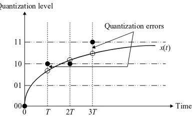
We can use 2 bits to define four equally spaced levels (00, 01, 10, and 11) to classify the signal into the four subranges as illustrated in Figure 1.5. In this figure, the symbol ‘o’ represents the discrete-time signalx(nT), and the symbol ‘
r
’ represents the digital signalx(n). The spacing between two consecutive quantization levels is called the quantization width, step, or resolution. If the spacing between these levels is the same, then we have a uniform quantizer. For the uniform quantization, the resolution is given by dividing a full-scale range with the number of quantization levels, 2B.In Figure 1.5, the difference between the quantized number and the original value is defined as the quantization error, which appears as noise in the converter output. It is also called the quantization noise, which is assumed to be random variables that are uniformly distributed. If aB-bit quantizer is used, the signal-to-quantization-noise ratio (SQNR) is approximated by (will be derived in Chapter 3)
SQNR≈6BdB. (1.5)
This is a theoretical maximum. In practice, the achievable SQNR will be less than this value due to imperfections in the fabrication of converters. However, Equation (1.5) still provides a simple guideline for determining the required bits for a given application. For each additional bit, a digital signal will have about 6-dB gain in SQNR. The problems of quantization and their solutions will be further discussed in Chapter 3.
Example 1.3:If the input signal varies between 0 and 5 V, we have the resolutions and SQNRs for the following commonly used data converters:
1. An 8-bit ADC with 256 (28) levels can only provide 19.5 mV resolution and 48 dB SQNR. 2. A 12-bit ADC has 4096 (212) levels of 1.22 mV resolution, and provides 72 dB SQNR.
0 T 2T 3T
00 01 10 11 Quantization level
Time
x(t) Quantization errors
3. A 16-bit ADC has 65 536 (216) levels, and thus provides 76.294μV resolution with 96 dB SQNR.
Obviously, with more quantization levels, one can represent analog signals more accurately. The dynamic range of speech signals is very large. If the uniform quantization scheme shown in Figure 1.5 can adequately represent loud sounds, most of the softer sounds may be pushed into the same small value. This means that soft sounds may not be distinguishable. To solve this problem, a quantizer whose quantization level varies according to the signal amplitude can be used. In practice, the nonuniform quantizer uses uniform levels, but the input signal is compressed first using a logarithm function. That is, the logarithm-scaled signal, rather than the original input signal itself, will be quantized. The compressed signal can be reconstructed by expanding it. The process of compression and expansion is called companding (compressing and expanding). For example, the ITU-T G.711μ-law (used in North America and parts of Northeast Asia) and A-law (used in Europe and most of the rest of the world) companding schemes are used in most digital telecommunications. The A-law companding scheme gives slightly better performance at high signal levels, while theμ-law is better at low levels.
As shown in Figure 1.1, the input signal to DSP hardware may be a digital signal from other DSP systems. In this case, the sampling rate of digital signals from other digital systems must be known. The signal processing techniques called interpolation and decimation can be used to increase or decrease the existing digital signals’ sampling rates. Sampling rate changes may be required in many multirate DSP systems such as interconnecting DSP systems that are operated at different rates.
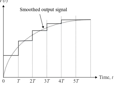
1.2.3 Smoothing Filters
Most commercial DACs are zero-order-hold devices, meaning they convert the input binary number to the corresponding voltage level and then hold that value forTs until the next sampling instant. Therefore, the DAC produces a staircase-shape analog waveformy′(t) as shown by the solid line in Figure 1.6, which is a rectangular waveform with amplitude equal to the input value and duration ofTs. Obviously, this staircase output contains some high-frequency components due to an abrupt change in signal levels. The reconstruction or smoothing filter shown in Figure 1.1 smoothes the staircase-like analog signal generated by the DAC. This lowpass filtering has the effect of rounding off the corners (high-frequency components) of the staircase signal and making it smoother, which is shown as a dotted line in Figure 1.6. This analog lowpass filter may have the same specifications as the antialiasing filter with cutoff frequencyfc≤ fs/2. High-quality DSP applications, such as professional digital audio, require the use
y′(t)
Time, t
0 T 2T 3T 4T 5T
Smoothed output signal
of reconstruction filters with very stringent specifications. To reduce the cost of using high-quality analog filter, the oversampling technique can be adopted to allow the use of low-cost filter with slower roll off.
1.2.4 Data Converters
There are two schemes of connecting ADC and DAC to DSP processors: serial and parallel. A parallel converter receives or transmits all theBbits in one pass, while the serial converters receive or transmit Bbits in a serial bit stream. Parallel converters must be attached to the DSP processor’s external address and data buses, which are also attached to many different types of devices. Serial converters can be connected directly to the built-in serial ports of DSP processors. This is why many practical DSP systems use serial ADCs and DACs.
Many applications use a single-chip device called an analog interface chip (AIC) or a coder/decoder (CODEC), which integrates an antialiasing filter, an ADC, a DAC, and a reconstruction filter all on a single piece of silicon. In this book, we will use Texas Instruments’ TLV320AIC23 (AIC23) chip on the DSP starter kit (DSK) for real-time experiments. Typical applications using CODEC include modems, speech systems, audio systems, and industrial controllers. Many standards that specify the nature of the CODEC have evolved for the purposes of switching and transmission. Some CODECs use a logarithmic quantizer, i.e., A-law orμ-law, which must be converted into a linear format for processing. DSP processors implement the required format conversion (compression or expansion) in hardware, or in software by using a lookup table or calculation.
The most popular commercially available ADCs are successive approximation, dual slope, flash, and sigma–delta. The successive-approximation ADC produces aB-bit output inBclock cycles by comparing the input waveform with the output of a DAC. This device uses a successive-approximation register to split the voltage range in half to determine where the input signal lies. According to the comparator result, 1 bit will be set or reset each time. This process proceeds from the most significant bit to the least significant bit. The successive-approximation type of ADC is generally accurate and fast at a relatively low cost. However, its ability to follow changes in the input signal is limited by its internal clock rate, and so it may be slow to respond to sudden changes in the input signal.
The dual-slope ADC uses an integrator connected to the input voltage and a reference voltage. The integrator starts at zero condition, and it is charged for a limited time. The integrator is then switched to a known negative reference voltage and charged in the opposite direction until it reaches zero volts again. Simultaneously, a digital counter starts to record the clock cycles. The number of counts required for the integrator output voltage to return to zero is directly proportional to the input voltage. This technique is very precise and can produce ADCs with high resolution. Since the integrator is used for input and reference voltages, any small variations in temperature and aging of components have little or no effect on these types of converters. However, they are very slow and generally cost more than successive-approximation ADCs.
A voltage divider made by resistors is used to set reference voltages at the flash ADC inputs. The major advantage of a flash ADC is its speed of conversion, which is simply the propagation delay of the comparators. Unfortunately, aB-bit ADC requires (2B−1) expensive comparators and laser-trimmed resistors. Therefore, commercially available flash ADCs usually have lower bits.
Analog input +
− Σ
Sigma
Delta
1-bit B-bit
1-bit DAC
1-bit ADC
∫
Digitaldecimator
Figure 1.7 A conceptual sigma–delta ADC block diagram
ADCs are high resolution and good noise characteristics at a competitive price because they use digital filters.
Example 1.4:In this book, we use the TMS320VC5510 DSK for real-time experiments. The C5510 DSK uses an AIC23 stereo CODEC for input and output of audio signals. The ADCs and DACs within the AIC23 use the multi-bit sigma–delta technology with integrated oversampling digital interpolation filters. It supports data wordlengths of 16, 20, 24, and 32 bits, with sampling rates from 8 to 96 kHz including the CD standard 44.1 kHz. Integrated analog features consist of stereo-line inputs and a stereo headphone amplifier with analog volume control. Its power management allows selective shutdown of CODEC functions, thus extending battery life in portable applications such as portable audio and video players and digital recorders.
1.3 DSP Hardware
DSP systems are required to perform intensive arithmetic operations such as multiplication and addition. These tasks may be implemented on microprocessors, microcontrollers, digital signal processors, or custom integrated circuits. The selection of appropriate hardware is determined by the applications, cost, or a combination of both. This section introduces different digital hardware implementations for DSP applications.
1.3.1 DSP Hardware Options
As shown in Figure 1.1, the processing of the digital signalx(n) is performed using the DSP hardware. Although it is possible to implement DSP algorithms on any digital computer, the real applications determine the optimum hardware platform. Five hardware platforms are widely used for DSP systems: 1. special-purpose (custom) chips such as application-specific integrated circuits (ASIC);
2. field-programmable gate arrays (FPGA);
Table 1.1 Summary of DSP hardware implementations
DSP processors with
ASIC FPGA μP/μC DSP processor HW accelerators
Flexibility None Limited High High Medium
Design time Long Medium Short Short Short
Power consumption Low Low–medium Medium–high Low–medium Low–medium
Performance High High Low–medium Medium–high High
Development cost High Medium Low Low Low
Production cost Low Low–medium Medium–high Low–medium Medium
ASIC devices are usually designed for specific tasks that require a lot of computations such as digital subscriber loop (DSL) modems, or high-volume products that use mature algorithms such as fast Fourier transform and Reed–Solomon codes. These devices are able to perform their limited functions much faster than general-purpose processors because of their dedicated architecture. These application-specific products enable the use of high-speed functions optimized in hardware, but they are deficient in the programmability to modify the algorithms and functions. They are suitable for implementing well-defined and well-tested DSP algorithms for high-volume products, or applications demanding extremely high speeds that can be achieved only by ASICs. Recently, the availability of core modules for some common DSP functions has simplified the ASIC design tasks, but the cost of prototyping an ASIC device, a longer design cycle, and the lack of standard development tools support and reprogramming flexibility sometimes outweigh their benefits.
FPGAs have been used in DSP applications for years as glue logics, bus bridges, and peripherals for re-ducing system costs and affording a higher level of system integration. Recently, FPGAs have been gaining considerable attention in high-performance DSP applications, and are emerging as coprocessors for stan-dard DSP processors that need specific accelerators. In these cases, FPGAs work in conjunction with DSP processors for integrating pre- and postprocessing functions. FPGAs provide tremendous computational power by using highly parallel architectures for very high performance. These devices are hardware re-configurable, thus allowing the system designer to optimize the hardware architectures for implementing algorithms that require higher performance and lower production cost. In addition, the designer can imple-ment high-performance complex DSP functions in a small fraction of the total device, and use the rest to implement system logic or interface functions, resulting in both lower costs and higher system integration.
Example 1.5:There are four major FPGA families that are targeted for DSP systems: Cyclone and Stratix from Altera, and Virtex and Spartan from Xilinx. The Xilinx Spartan-3 FPGA family (introduced in 2003) uses 90-nm manufacturing technique to achieve low silicon die costs. To support DSP functions in an area-efficient manner, Spartan-3 includes the following features:
r
embedded 18×18 multipliers;r
distributed RAM for local storage of DSP coefficients;r
16-bit shift register for capturing high-speed data; andr
large block RAM for buffers.Program
memory Processor
Program address bus
Program data bus
Data address bus
Data memory
Data data bus
(a) Harvard architecture
Memory Processor
Address bus
Data bus
(b) von Newmann architecture
Figure 1.8 Different memory architectures: (a) Harvard architecture; (b) von Newmann architecture
General-purposeμP/μC becomes faster and increasingly able to handle some DSP applications. Many electronic products are currently designed using these processors. For example, automotive controllers use microcontrollers for engine, brake, and suspension control. If a DSP application is added to an existing product that already contains aμP/μC, it is desired to add the new functions in software without requiring an additional DSP processor. For example, Intel has adopted a native signal processing initiative that uses the host processor in computers to perform audio coding and decoding, sound synthesis, and so on. Software development tools forμP/μC devices are generally more sophisticated and powerful than those available for DSP processors, thus easing development for some applications that are less demanding on the performance and power consumption of processors.
General architectures ofμP/μC fall into two categories: Harvard architecture and von Neumann archi-tecture. As illustrated in Figure 1.8(a), Harvard architecture has a separate memory space for the program and the data, so that both memories can be accessed simultaneously. The von Neumann architecture as-sumes that there is no intrinsic difference between the instructions and the data, as illustrated in Figure 1.8(b). Operations such as add, move, and subtract are easy to perform onμPs/μCs. However, complex instructions such as multiplication and division are slow since they need a series of shift, addition, or subtraction operations. These devices do not have the architecture or the on-chip facilities required for efficient DSP operations. Their real-time DSP performance does not compare well with even the cheaper general-purpose DSP processors, and they would not be a cost-effective or power-efficient solution for many DSP applications.
It is important to note that some microprocessors such as Pentium add multimedia exten-sion (MMX) and streaming single-instruction, multiple-data (SIMD) extenexten-sion to support DSP operations. They can run in high speed (>3 GHz), provide single-cycle multiplication and arith-metic operations, have good memory bandwidth, and have many supporting tools and software available for easing development.
A DSP processor is basically a microprocessor optimized for processing repetitive numerically inten-sive operations at high rates. DSP processors with architectures and instruction sets specifically designed for DSP applications are manufactured by Texas Instruments, Freescale, Agere, Analog Devices, and many others. The rapid growth and the exploitation of DSP technology is not a surprise, considering the commercial advantages in terms of the fast, flexible, low power consumption, and potentially low-cost design capabilities offered by these devices. In comparison to ASIC and FPGA solutions, DSP processors have advantages in easing development and being reprogrammable in the field to allow a product feature upgrade or bug fix. They are often more cost-effective than custom hardware such as ASIC and FPGA, especially for low-volume applications. In comparison to the general-purposeμP/μC, DSP processors have better speed, better energy efficiency, and lower cost.
In many practical applications, designers are facing challenges of implementing complex algorithms that require more processing power than the DSP processors in use are capable of providing. For exam-ple, multimedia on wireless and portable devices requires efficient multimedia compression algorithms. The study of most prevalent imaging coding/decoding algorithms shows some DSP functions used for multimedia compression algorithms that account for approximately 80 % of the processing load. These common functions are discrete cosine transform (DCT), inverse DCT, pixel interpolation, motion es-timation, and quantization, etc. The hardware extension or accelerator lets the DSP processor achieve high-bandwidth performance for applications such as streaming video and interactive gaming on a sin-gle device. The TMS320C5510 DSP used by this book consists of the hardware extensions that are specifically designed to support multimedia applications. In addition, Altera has also added the hardware accelerator into its FPGA as coprocessors to enhance the DSP processing abilities.
Today, DSP processors have become the foundation of many new markets beyond the traditional signal processing areas for technologies and innovations in motor and motion control, automotive systems, home appliances, consumer electronics, and vast range of communication systems and devices. These general-purpose-programmable DSP processors are supported by integrated software development tools that include C compilers, assemblers, optimizers, linkers, debuggers, simulators, and emulators. In this book, we use Texas Instruments’ TMS320C55x for hands-on experiments. This high-performance and ultralow power consumption DSP processor will be introduced in Chapter 2. In the following section, we will briefly introduce some widely used DSP processors.
1.3.2 DSP Processors
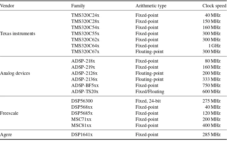
In 1979, Intel introduced the 2920, a 25-bit integer processor with a 400 ns instruction cycle and a 25-bit arithmetic-logic unit (ALU) for DSP applications. In 1982, Texas Instruments introduced the TMS32010, a 16-bit fixed-point processor with a 16×16 hardware multiplier and a 32-bit ALU and accumulator. This first commercially successful DSP processor was followed by the development of faster products and floating-point processors. The performance and price range among DSP processors vary widely. Today, dozens of DSP processor families are commercially available. Table 1.2 summarizes some of the most popular DSP processors.
Table 1.2 Current commercially available DSP processors
Vendor Family Arithmetic type Clock speed
TMS320C24x Fixed-point 40 MHz
TMS320C28x Fixed-point 150 MHz
TMS320C54x Fixed-point 160 MHz
Texas instruments TMS320C55x Fixed-point 300 MHz
TMS320C62x Fixed-point 300 MHz
TMS320C64x Fixed-point 1 GHz
TMS320C67x Floating-point 300 MHz
ADSP-218x Fixed-point 80 MHz
ADSP-219x Fixed-point 160 MHz
Analog devices ADSP-2126x Floating-point 200 MHz
ADSP-2136x Floating-point 333 MHz
ADSP-BF5xx Fixed-point 750 MHz
ADSP-TS20x Fixed/Floating 600 MHz
DSP56300 Fixed, 24-bit 275 MHz
DSP568xx Fixed-point 40 MHz
Freescale DSP5685x Fixed-point 120 MHz
MSC71xx Fixed-point 200 MHz
MSC81xx Fixed-point 400 MHz
Agere DSP1641x Fixed-point 285 MHz
Source: Adapted from [11]
pointers. They provide good performance with modest power consumption and memory usage, thus are widely used in automotives, appliances, hard disk drives, modems, and consumer electronics. For exam-ple, the TMS320C2000 and DSP568xx families are optimized for control applications, such as motor and automobile control, by integrating many microcontroller features and peripherals on the chip.
The midrange processor group includes Texas Instruments’ TMS320C5000 (C54x and C55x), Analog Devices’ ADSP219x and ADSP-BF5xx, and Freescale’s DSP563xx. These enhanced processors achieve higher performance through a combination of increased clock rates and more advanced architectures. These families often include deeper pipelines, instruction cache, complex instruction words, multiple data buses (to access several data words per clock cycle), additional hardware accelerators, and parallel execution units to allow more operations to be executed in parallel. For example, the TMS320C55x has two multiply–accumulate (MAC) units. These midrange processors provide better performance with lower power consumption, thus are typically used in portable applications such as cellular phones and wireless devices, digital cameras, audio and video players, and digital hearing aids.
These conventional and enhanced DSP processors have the following features for common DSP algorithms such as filtering: