introduction to real analysis third edition robert g bartle and donald r sherbert

INTRODUCTION TO REAL ANALYSIS

Third Edition

Robert G. Bartle

Donald R. Sherbert

Easten Michigan University, Ypsilanti University of Illinois, Urbana-Champaign

ACQUISITION EDITOR ASSOCIATE EDITOR PRODUCTION EDITOR PHOTO EDITOR

ILUS TRATION COORDINATOR

Barbara Holland Sharon Prendergast Ken Santor Nicole Horlacher Gene Aiello

This book was set in Times Roman by Eigentype Compositors, and printed and bound by Hamilton Printing Company. The cover was printed by Phoenix Color Corporation.

This book is printed on acid-free paper. §

The paper in this book was manufactured by a mill whose forest management programs include sustained yield harvesting of its timberlands. Sustained yield harvesting principles ensure that the numbers of trees CUI each year does not exceed the amount of new growth.

Copyright © 2000 John Wiley & Sons, Inc. All rights reserved.

No part of this publication may be reproduced, stored in a retrieval system or transmitted

in any form or by any means, electronic, mechanical, photocopying, recording, scanning

or otherwise, except as permitted under Section 107 or 108 of the 1976 United States Copyright Act, without either the prior written permission of the Publisher, or authorization through payment of the appropriate per-copy fee to the Copyright Clearance Center,

222 Rosewood Drive, Danvers, MA 01923, (508) 750-8400, fx (508) 750-4470.

Requests to the Publisher for permission should be addressed to the Permissions Department, John Wiley & Sons, Inc., 05 Third Avenue, New York, Y 10158-012,

(212) 850-601 1, fax (212) 850-6008, E-Mail: PERMRE@LE.COM.

Libray of Congress Caaloging in ublication Daa:

Bartle, Robert Gardner,

1927-Introduction to real analysis / Robert G. Bartle, Donald R., Sherbert. - 3rd ed. p. cm.

Includes bibliographical references and index. ISBN 0-47 1-32148-6 (a1k. paper)

1. Mathematical analysis. 2. Functions of real variables.

1. Sherbert, Donald R., 1935- . II. Title. QA300.B294 2000

515-dc21

A. M. S. Classiication 26-01

Printed in the United States of America

20 19 18 17 16 15 14 13 12 II

99-13829

PREFACE

The study of real analysis is indispensible for a prospective graduate student of pure or

applied mathematics. It also has great value for any undergraduate student who wishes

to go beyond the routine manipulations of formulas to solve standard problems, because

it develops the ability to think deductively, analyze mathematical situations, and extend

ideas to a new context.

n

recent years, mathematics has become valuable in many areas,

including economics and management science as well as the physical sciences, engineering,

and computer science. Our goal is to provide an accessible, reasonably paced textbook in

the undamental concepts and techniques of real analysis for students in these areas. This

book is designed for students who have studied calculus as it is raditionally presented in

the United States. While students ind this book challenging, our experience is that serious

students at this level are fully capable of mastering the material presented here.

The irst two editions of this book were very well received, and we have taken pains

to maintain the same spirit and user-friendly approach. In preparing this edition, we have

examined every section and set of exercises, sreamlined some arguments, provided a few

new examples, moved certain topics to new locations, and made revisions. Except for the

new Chapter

10,

which deals with the generalized Riemann integral, we have not added

much new material. While there is more materil than can be covered in one semester,

instructors may wish to use certain topics as honors projects or extra credit assignments.

It is desirable that the student have had some exposure to proofs, but we do not assume

that to be the case. To provide some help for students in analyzing proofs of theorems,

we include an appendix on "Logic and Proofs" that discusses topics such as implications,

quantifiers, negations, contrapositives, and diferent types of proofs. We have kept the

discussion informal to avoid becoming mired in the technical details of formal logic. We

feel that it is a more useful experience to len how to construct proofs by irst watching

and then doing than by reading about techniques of proof.

We have adopted a medium level of generality consistently throughout the book: we

present results that are general enough to cover cases that actually arise, but we do not strive

for maximum generality. In the main, we proceed from the particular to the general. Thus

we consider continuous functions on open and closed intervals in detail, but we are careul

to present proofs that can readily be adapted to a more general situation. (In Chapter

1 1

we take particular advantage of the approach.) We believe that it is important to provide

students with many examples to aid them in their understanding, and we have compiled

rather extensive lists of exercises to challenge them. While we do leave routine proofs as

exercises, we do not try to attain brevity by relegating diicult proofs to the exercises.

owever, in some of the later sections, we do break down a moderately difficult exercise

into a sequence of steps.

In Chapter

1

we present a brief summary of the notions and notations for sets and

functions that we use.

A

discussion of Mathematical Induction is also given, since inductive

proofs arise frequently. We also include a short section on finite, countable and infinite sets.

We recommend that this chapter be covered quickly, or used as background material,

retuning later as necessary.

vi PREFACE

Chapter

2

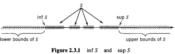
presents the properties of the real number system . The irst two sections deal with the Algebraic and Order Properties and provide some practice in writing proofs of elementry results. The crucial Completeness Property is given in Section 2.3 as the Supremum Property, and its ramifications are discussed throughout the remainder of this chapter.

In Chapter

3

we give a thorough treatment of sequences in

R

and the associated limit concepts. The material is of the greatest importance; fortunately, students find it rather natural although it takes some time for them to become fully accustomed to the use of €.

In the new Section 3.7, we give a brief introduction to infinite series, so that this important topic will not be omitted due to a shortage of time.

Chapter

4

on limits of functions and Chapter

5

on continuous functions constitute the heart of the book. Our discussion of limits and continuity relies heavily on the use of sequences, and the closely parallel approach of these chapters reinforces the understanding of these essential topics. The fundamental properties of continuous functions (on intervals) are discussed in Section

5.3

and

5.4.

The notion of a "gauge" is introduced in Section

5.5

and used to give altenative proofs of these properties. Monotone functions are discussed in Section

5.6.

The basic theory of the derivative is given in the first part of Chapter

6.

This important material is standard, except that we have used a result of Caratheodory to give simpler proofs of the Chain Rule and the Inversion Theorem. The remainder of this chapter consists of applications of the Mean Value Theorem and may be explored as time permits.

Chapter

7,

dealing with the Riemann integral, has been completely revised in this edition. Rather than introducing upper and lower integrals (as we did in the previous editions), we here define the integral as a limit of Riemann sums. This has the advantage that it is consistent with the students' irst exposure to the integral in calculus and in applications; since it is not dependent on order properties, it permits immediate generalization to complex­ and vector-valued functions that students may encounter in later courses. Contrary to popular opinion, this limit approach is no more dificult than the order approach. It also is consistent with the generalized Riemann integral that is discussed in detail in Chapter

10.

Section 7.4 gives a brief discussion of the familiar numerical methods of calculating the integral of continuous functions.

Sequences of functions and uniform convergence are discussed in the irst two sec­ tions of Chapter 8, and the basic transcendental functions are put on a firm foundation in Section 8.3 and 8.4 by using uniform convergence. Chapter

9

completes our discussion of ininite series. Chapters 8 and

9

are intrinsically important, and they also show how the material in the earlier chapters can be applied.

Chapter

10

is completely new; it is a presentation of the generalized Riemann integral (sometimes called the "Henstock-Kurzweil" or the "gauge" integral). It will be new to many readers, and we think they will be amazed that such an apparently minor modification of the deinition of the Riemann integral can lead to an integral that is more general than the Lebesgue integral. We believe that this relatively new approach to integration theory is both accessible and exciting to anyone who has studied the basic Riemann integral.

The final Chapter 1 1 deals with topological concepts. Earlier proofs given for intervals

are extended to a more abstract setting. For example, the concept of compactness is given proper emphasis and metric spaces are introduced. This chapter will be very useful for students continuing to graduate courses in mathematics.

PREFACE vii

We have provided rather lengthy lists of exercises, some easy and some challenging. We have provided "hints" for many of these exercises, to help students get started toward a solution or to check their "answer". More complete solutions of almost every exercise are given in a separate Instructor's Manual, which is available to teachers upon request to the publisher.

It is a satisfying experience to see how the mathematical maturity of the students increases and how the students gradually len to work comfortably with concepts that initially seemed so mysterious. But there is no doubt that a lot of hard work is required on the part of both the students and the teachers.

In order to enrich the historical perspective of he book, we include brief biographical sketches of some famous mathematicians who contributed to this area. We are particularly indebted to Dr. Patrick Muldowney for providing us with his photograph of Professors Henstock and Kurzweil. We also thank John Wiley & Sons for obtaining photographs of the other mathematicians.

To our wives, Carolyn and Janice, with our appreciation for their

CONTENTS

CHAPTER 1 PRELIMINARIES 1

1.1

Sets and Functions· 1

1.2

Mathematical Induction 12

1.3

Finite and Ininite Sets 16

CHAPTER 2 THE REAL NUMBERS 22

2.1

The Algebraic and Order Properties of

R

22

2.2

Absolute Value and Real Line 31

2.3

The Completeness Property of

R

34

2.4

Applications of the Supremum Property 38

2.5

Intervals 44

CHAPTER 3 SEQUENCES AND SERIES 52

3.1

Sequences and Their Limits 53

3.2

Limit Theorems 60

3.3

Monotone Sequences 68

3.4

Subsequences and the Bolzano-Weierstrass Theorem 75

3.5

The Cauchy Criterion 80

3.6

Properly Divergent Sequences 86

3.7

Introduction to Ininite Series 89

CHAPTER 4 LIMITS 96

4.1

Limits of Functions 97

4.2

Limit Theorems 105

4.3

Some Extensions of the Limit Concept 1 1 1

C.HAPTER 5 CONTINUOUS FUNCTIONS 119

5.1

Continuous Functions 120

5.2

Combinations of Continuous Functions 125

5.3

Continuous Functions on Intervals 129

5.4

Uniform Continuity 136

5.5

Continuity and Gauges 145

5.6

Monotone and Inverse Functions 149

x CONTENTS

CHAPTER 6 DIFFERENTIATION 157

6.1

The Derivative

158

6.2

The Mean Value Theorem

168

6.3

L'Hospital's Rules

176

6.4

Taylor's Theorem

183

CHAPTER 7 TE RIEMANN INTEGRAL 193

7.1

The Riemann Integral

194

7.2

Riemann Integrable Functions

202

7.3

The Fundamental Theorem

210

7.4

Approximate Integration

219

CHAPTER 8 SEQUENCES OF FUNCTIONS 227

8.1

Pointwise and Uniform Convergence

227

8.2

Interchange of Limits

233

8.3

The Exponential and Logarithmic Functions

239

8.4

The Trigonometric Functions

246

CHAPTER 9 INFINITE SERIES 253

9.1

Absolute Convergence

253

9.2

Tests for Absolute Convergence

257

9.3

Tests for Nonabsolute Convergence

263

9.4

Series of Functions

266

CHAPTER 10 THE GENERALIZED RIEMANN INTEGRAL 274

10.1

Definition and Main Properties

275

10.2

Improper and Lebesgue Integrals

287

10.3

Infinite Intervals

294

10.4

Convergence Theorems

301

CHAPTER 11 A GLIMPSE INTO TOPOLOGY 312

1 1.1

Open and Closed Sets in

R 312

1 1.2

Compact Sets

319

1 1.3

Continuous Functions

323

1 1.4

Metric Spaces

327

APPENDIX A LOGIC AND PROOFS 334

APPENDIX B FINITE AND COUNTABLE SETS 343

CONTENTS xi

APPENDIX D APPROXIMATE INTEGRATION 351

APPENDIX E TWO EXAMPLES 354

REFERENCES 357

PHOTO CREDITS 358

HINTS FOR SELECTED EXERCISES 359

CHAPTER 1

PRELIMINARIES

In this initial chapter we will present the background needed for the study of real analysis.

Section

1.1

consists of a brief survey of set operations and functions, two vital tools for all

of mathematics. In it we establish the notation and state the basic deinitions and properties

that will be used throughout the book. We will regard the word "set" as synonymous with

the words "class", "collection", and "family", and we will not deine these terms or give a

list of axioms for set theory. This approach, often referred to as "naive" set theory, is quite

adequate for working with sets in the context of real analysis.

Section

1.2

is concened with a special method of proof called Mathematical Induction.

t

is related to the fundamental properties of the natural number system and, though it is

restricted to proving particular types of statements, it is important and used frequently. An

informal discussion of the diferent types of proofs that are used in mathematics, such as

contrapositives and proofs by contradiction, can be found in Appendix A.

In Section

1.3

we apply some of the tools presented in the irst two sections of this

chapter to a discussion of what it means for a set to be inite or ininite. Creful deinitions

are given and some basic consequences of these deinitions are derived. The important

result that the set of rational numbers is countably ininite is established.

In addition to introducing basic concepts and establishing terminology and notation,

this chapter also provides the reader with some initial experience in working with precise

deinitions and writing proofs. The careul study of real analysis unavoidably entails the

reading and writing of proofs, and like any skill, it is necessary to practice. This chapter is

a starting point.

Section 1.1 Sets and Functions

To the reader:

In this section we give a brief review of the terminology and notation that

will be used in this text. We suggest that you look through quickly and come back later

when you need to recall the meaning of a term or a symbol.

If an element

x

is in a set

A,

we write

XEA

and say that

x

is a

member

of

A,

or that

x belongs

to

A.

If

x

is

not

in

A,

we write

x

¢ A.

If�very element of a set

A

also belongs to a set

B,

we say that

A

is a

subset

of

B

and write

or

We say that a set

A

is a

proper subset

of a set

B

if

A

� B,

but there is at least one element

of

B

that is not in

A.

In this case we sometimes write

A

C B.

2 CHAPTER 1 PRELINARlES

1.1.1 Deinition

wo sets

A

and

B

are said to be

equal.

and we write

A

=

B.

if they

contain the same elements.

Thus. to prove hat the sets

A

and

B

are equal. we must show that

A � B

and

B � A.

A

set is normally deined by either listing its elements explicitly. or by specifying a

property that determines he elements of the set. If

P

denotes a property that is meaningful

and unambiguous for elements of a set

S.

then we write

{x E

S

:

P(x)}

for the set of all elements

x

in

S

for which the property

P

is true. If the set

S

is understood

rom the context. then it is oten omitted in this notation.

Several special sets are used throughout this book. and they are denoted by standard

symbols. le will use the symbol

:=

to mean that the symbol on the left is being

deined

by the symbol on the right.)

•

The set of

natural numbers

N

:=

{I. 2. 3

•. . .

}.

•

The set of

integers Z := to.

1.

-1.2, -2, · · .},

•

The set

ofrational numbers Q : =

{min : m, n E

Z

and

n - OJ.

•

The set of

real numbers R

The set

R

of real numbers is of fundamental importance for us and will be discussed

at length in Chapter

2.

1.1.2 Examples (a)

The set

{x E N : x2 - 3x

+

2

=

O}

consists of those natural numbers satisfying the stated equation. Since the only solutions of

this quadratic equation re

x

=

1

and

x

=

2,

we can denote this set more simply by

{I, 2}.

(b) A

natural number

n

is

even

if it has the form

n

=

2k

for some

k E N.

The set of even

natural numbers can be written

{2k : k E N},

which is less cumbersome than

{n E N : n

=

2k, k E N}.

Similarly, the set of

odd

natural

numbers can be written

{2k - 1

:

k E N}.

o

Set Operations

We now deine the methods of obtaining new sets from given ones. Note that these set

operations are based on the meaning of the words "or", "and", and "not". For the union,

it is important to be aware of the fact that the word "or" is used in the

inclusive sense,

allowing the possibility that

x

may belong to both sets. In legal terminology, this inclusive

sense is sometimes indicated by "andlor".

1.1.3 Deinition (a)

The

union

of sets

A

and

B

is the set

1.1 SETS AND FUNCTIONS 3

(b) The intersection of the sets

A

and

B

is the set

A

n

B

:=

{x : x

E

A

and

x

E

B} .

(c) The complement of

B

relative to

A

is the set

A \B

:=

{x : x

E

A

and

x

t

B} .

A U B ID

Fiure 1.1.1 (a) A U B (b) A n B (c) A\B

A\B �

The set that has no elements is called the empty set and is denoted by the symbol 0.

Two sets

A

and

B

are said to be disjoint if they have no elements in common; this can be expressed by writing

A

n

B

= 0.

To illustrate the method of proving set equalities, we will next establish one of the

DeMorgan laws

for three sets. The proof of the other one is let as an exercise.

1.1.4 Theorem f

A, B, C

re sets, then (a)

A\(B

U

C)

=

(A\B)

n

(A\C),

(b)

A\(B

n

C)

=

(A\B)

U

(A\C).

Proo. To prove (a), we will show that every element in

A \ (B

U

C)

is contained in both

(A \B)

and

(A \C),

and conversely.

If

x

is in

A\(B

U

C),

then

x

is in

A,

but

x

is not in

B

U

C.

Hence

x

is in

A,

but

x

is neither in

B

nor in

C.

Therefore,

x

is in

A

but not

B,

and

x

is in

A

but not

C.

Thus,

x

E

A \B

and

x

E

A \C,

which shows that

x

E

(A \B)

n

(A \C).

Conversely, if

x

E

(A\B)

n

(A\C),

then

x

E

(A\B)

and

x

E

(A\C).

Hence

x

E

A

and both

x

t

B

and

x

t

C.

Therefore,

x

E

A

and

x

t

(B

U

C),

so that

x

E

A \ (B

U

C).

Since the sets

(A \B)

n

(A \ C)

and

A \ (B

U

C)

contain the same elements, they are

equal by Deinition

1.1.1.

Q.E.D.

There are times when it is desirable to form unions and intersections of more than two sets. For a finite collection of sets

{AI' A2, .. . , An},

their union is the set

A

consisting of all elements that belong to

at least one

of the sets

Ak,

and their intersection consists of all el�ments that belong to

all

of the sets

Ak•

This is extended to an ininite collection of sets

{A

_I'

A2, ••• , An' . . . }

as follows. Their

union is the set of elements that belong to

at least one

of the sets

An'

In this case we write

0

4 CHTER 1 PRELIMNARIES

Similarly, their

intersection

is the set of elements that belong to

all

of these sets

_An'

In this

case we write

0

n

An :=

{x : x

E

An

for all

n E N} .

n=l

Cartesian Products

In order to discuss unctions, we deine the Cartesian product of two sets.

1.1.5 Deinition

If

A

and B are nonempty sets, then the

Cartesian product A x

B of

A

and B is the set of all ordered pairs

(a, b)

with

a E

A

and

b E

B.

That is,

A x

B

: =

{(a, b) : a E

A,

bE B} .

Thus if

A =

{l, 2, 3}

and

B

=

{I, 5},

then the set

A x

B is the set whose elements are

the ordered pairs

(1, 1), (1, 5), (2, 1), (2, 5), (3, 1), (3, 5).

We may visualize the set

A x

B as the set of six points in the plane with the coordinates

that we have just listed.

We oten draw a diagram (such as Figure

1.1.2)

to indicate the Cartesian product of

two sets

A

and

B.

However, it should be realized that this diagram may be a simplification.

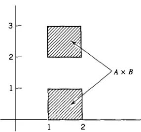
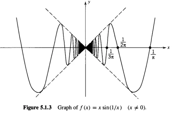
For example, if

A :=

{

x

E

R

:

1

:::

x

:::

2}

and B

:=

{y E

R

:

0

:::

y

::: 1

or

2 ::: y ::: 3},

then instead of a rectangle, we should have a drawing such as Figure

1.1.3.

We will now discuss the undamental notion of

afunction

or a

mapping.

To the mathematician of the early nineteenth century, the word "function" meant a

deinite formula, such as f(x)

:=

x2

+

3x

- 5,

which associates to each real number

x

another number

f(x).

(Here,

f(O)

=

-5, f(1)

=

-1, f(5)

=

35.)

This understanding

excluded the case of diferent formulas on diferent intervals, so that unctions could not

be deined "in pieces".

B

b ---1(a, b)

I I I I I

a

AxB

A

Figure 1.1.2

3

2

AxB

2

1.1 SETS AD UNCTIONS 5

As mathematics developed, it became clear that a more general definition of "function" would be useful. It also became evident that it is important to make a clear distinction between the function itself and the values of the function. A revised definition might be:

A function f from a set A into a set B is a rule of correspondence that assigns to each element x in A a uniquely determined element f (x) in B.

But however suggestive this revised deinition might be, there is the difficulty o f interpreting the phrase "rule of correspondence". In order to clarify this, we will express the definition entirely in terms of sets; in efect, we will define a function to be its graph. While this has the disadvantage of being somewhat artificial, it has the advantage of being unambiguous and clearer.

1.1.6 Deinition Let A and B be sets. Then a function from A to B is a set f of ordered pairs in A x B such that for each

a

E A there exists a unique

b

E B with

(a, b)

E f. (In other words, if

(a, b)

E f and

(a, b')

E f, then

b = b'.)

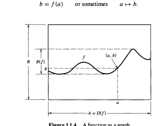
The set A of first elements of a function f is called the domain of f and is often denoted by D(f). The set of all second elements in f is called the range of f and is often denoted by R(f). Note that, although D(f)

=

A, we only have R(f) � B. (See Figure 1.1.4.)

The essential condition that:

(a, b)

E f and

(a, b')

E f implies that

b= b'

is sometimes called the

vertical line test.

In geometrical terms it says every vertical line

x

= a

with

a

E A intersects the graph of f exactly once. The notation

f : A;B

is often used to indicate that f is a function from A into B. We will also say that f is a mapping of A into

B,

or that f maps A into B. If

(a, b)

is an element in f, it is customary to write

b = f(a)

or sometimes

a

+

b.

6 CHAPTER 1 PRELIMINARIES

If

b

=

f(a),

we often refer to

b

as the value of

f

at

a,

or as the image of

a

under

f.

ransformations and Machines

Aside from using graphs, we can visualize a function as a

tansformation

of the set DU) = A into the set RU) � B. In this phraseology, when

(a, b)

E

f,

we think of

f

as taking the element

a

from A and "ransforming" or "mapping" it into an element

b

=

f(a)

in

RU) � B. We often draw a diagram, such as Figure

1.1.5,

even when the sets A and B are not subsets of the plane.

b =!(a)

Figue 1.1.5 A unction as a transfonnation

Rf)

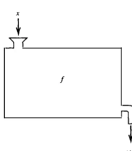
There is another way of visualizing a function: namely, as a

machine

that accepts elements of DU) = A as

inputs

and produces corresponding elements of RU) � B as

outputs.

f we take an element x E D U) and put it into

f,

then out comes the corresponding value

f(x).

If we put a diferent element y E DU) into

f,

then out comes

f

ey) which may or may not difer rom

f(x).

If we ry to insert something that does not belong to DU) into

f,

we find that it is not accepted, for

f

can operate only on elements from DU). (See Figure

1.1.6.)

This last visualization makes clear the distinction between

f

and

f (x):

the first is the machine itself, and the second is the output of the machine

f

when

x

is the input. Whereas no one is likely to confuse a meat grinder with ground meat, enough people have confused functions with their values that it is worth distinguishing between them notationally.

x

!

!(x)

1.1 SETS AND UNCTIONS 7

Direct and Inverse Images

Let

f

: A � B be a function with domain

DC!)

= A and range

RC!)

� B.

1.1.7 Deinition If

E

is a subset of A, then the direct image of

E

under

f

is the subset

f(E)

of B given by

f(E)

:=

{f(x) : x

E

E

} .

If

H

is a subset of B, then the inverse image of

H

under

f

is the subset

f -, (H)

of A

given by

f-'(H)

:=

{x

E A

: f(x)

E

H

} .

Remark The notation

f-' (H)

used in this connection has its disadvantages. However, we will use it since it is the standard notation.

Thus, if we are given a set

E

� A, then a point

y,

E B is in the direct image

f(E)

if and only if there exists at least one point

x,

E

E

such that Y, =

f(x,).

Similarly, given

a set

H

� B, then a point

x2

is in the inverse image

f-'(H)

if and only if Y

2

: =

f(x2)

belongs to

H.

(See Figure 1 . 1 .7.)

1.1.8 Examples (a) Let

f

:

R

�

R

be deined by

f(x)

:=

x2•

Then the direct image

of the set

E

:=

{x :

0

�

x

� 2} is the set

f(E)

=

{y

:

0

� Y � 4}.

If

G

:=

{y

: 0

� Y � 4}, then the inverse image of

G

is the set

f-'(G)

=

{x :

-2 �

x

� 2}. Thus, in this case, we see that

f-' C!(E»

=

E.

On the other hand, we have

f (J-'(G»)

=

G.

But if

H

:=

{y

: -1 � Y � I}, then

we have

f (J-' (H»)

=

{y

:

0

�

y

� I } =

H.

A sketch of the graph of

f

may help to visualize these sets.

(b) Let

f

: A � B, and let

G, H

be subsets of B. We will show that

f-'(G

n

H)

�

f-'(G)

n

f-'(H).

For, if

x

E

f-'(G

n

H),

then

f(x)

E

G

n

H,

so that

f(x)

E

G

and

f(x)

E

H.

But this implies that

x

E

f-'(G)

and

x

E

f-'(H),

whence

x

E

f-'(G)

n

f-'(H).

Thus the stated implication is proved. [The opposite inclusion is also true, so that we actually have set

equality between these sets; see Exercise 13.] 0

Further facts about direct and inverse images are given in the exercises.

E

f �

H

8 CHAPTER 1 PRELIMINARIES

Special ypes of Functions

The following deinitions identify some very important types of functions.

1.1.9 Deinition Let I : A + B be a unction from A to B.

(a) The function I is said to be ijective (or to be one-one) if whenever x, = x2, then I(x,) = l(x2)· f I is an injective function, we also say that I is an ijection. (b) The function I is said to be surjective (or to map A onto B) if I(A) = B; that is, if

the range

R(f)

= B. If I is a surjective function, we also say that I is a surjection. (c) If I is both injective and sujective, then I is said to be bijective. If I is bijective, we

also say that I is a bijection.

• In order to prove that a function I is injective, we must establish that: for all x" x2 in A, if I(x,) = l(x2), then x, = x2• To do this we assume that I(x,) = l(x2) and show that x, = x2.

[In other words, the graph of I satisies the

irst horizontal line test:

Every horizontal line y =

b

with

b

E B intersects the graph I in

at most

one point.]

• To prove that a function I is sujective, we must show that for any

b E

B there exists at least one x E A such that I (x) =

b.

[In other words, the graph of I satisies the

second horizontal line test:

Every horizontal line y =

b

with

b

E B intersects the graph I in

at least

one point.]

1.1.10 Example Let A := {x E R : x = l } and deine /(x) := 2x/(x -l) for allx

E

A. To show that I is injective, we take x, and x2 in A and assume that I(x,) = l(x2). Thus we have

2x, _2x2

- = -,

x, -

1

_x2 -

1

which implies that x, (x2 - 1) = x2(x, -1), and hence x, = x2. Therefore I is injective.

To determine the range of I, we solve the equation y = 2x/(x -

1)

for x in tenus of

y. We obtain x = y / (y - 2), which is meaningful for y = 2. Thus the range of I is the set B := {y E R : y

=

2}. Thus, I is a bijection of A onto B. 0

Inverse Functions

If I is a function from A into B, then I is a special subset of A x B (namely, one passing

the

vertical line test.)

The set of ordered pairs in B x A obtained by interchanging the

members of ordered pairs in I is not generally a function. (That is, the set I may not pass

both

of the

horizontal line tests.)

However, if I is a bijection, then this interchange does lead to a function, called the "inverse function" of I.

1.1.11 Deinition If I : A + B is a bijection of A onto B, then

g :=

feb, a)

E B x A :

(a, b)

E

f}

1.1 SETS AND UNCTIONS 9

We can also express the connection between

I

and its inverse

I-I

by noting that

D(f)

=

R(f-I)

and

R(f)

=

D(f-I)

_{and that}

b

=

I(a)

if and only if

a

=

I-I(b).

For example, we saw in Example

1.1.10

that the function

2x

I(x)

: =

x - I

is a bijection of A :=

{x E

R :

x

=

I}

onto the set B :=

{y E

R :

y

=

2}.

The function

inverse to I is given by

I-I(y)

:=

y - 2

for

y

E B.

Remark We introduced the notation

I-I (H)

in Deinition

1.1.7.

It makes sense even if

I

does not have an inverse unction. However, if the inverse function

I-I

does exist, then

I-I (H)

is the direct image of the set

H

� B under

I-I.

Composition of Functions

It often happens that we want to "compose" two functions

I, g

by first inding

I (x)

and then applying

g

to get

g (f (x));

however, this is possible only when

I (x)

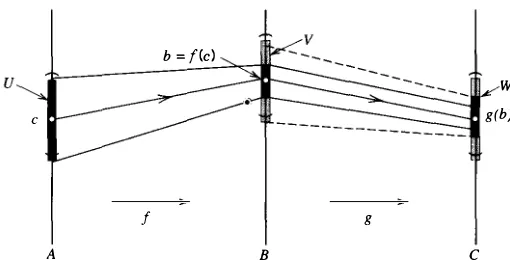
belongs to the domain of

g.

In order to be able to do this for

all I(x),

we must assume that the range of

I

is contained in the domain of

g.

(See Figure

1.1.8.)

1.1.12 Deinition If

I

: A � B and

g

: B �

C,

and if

R(f)

�

D(g)

= B, then the composite function

g o

I (note the orderl) is the function from A into

C

deined by

(g

0

f)(x)

:=

g(f(x))

for ll

x

E A.

1.1.13 Examples (a) The order of the composition must be careully noted. For, let

I

and

g

be the functions whose values at

x E

R are given by

I(x)

:=

2x

and

g(x)

:=

3x2

-

1.

Since

D(g)

= R and

R(f)

� R =

D(g),

then the domain

D(g

₀

f)

is also equal to R , and

the composite function

g

0 I is given by

A

(g

0

f)(x)

=

3(2x)2

_-

1

=

12x2

-

1.

I �

B

gol

10 CHAPTER 1 PRELIMINARIES

On the other hand, the domain of the composite function

l o g

is also R, but

(f

0

g)(x) = 2(3x2 - 1) = 6x2

-

2.

Thus, in this case, we have

g

0

I

=

l o g.

(b) In considering

g

0

I,

some care must be exercised to be sure that the range of 1 is

contained in the domain of

g.

For example, if

I(x) := l - x2

and

g(x) :=

X,

then, since

D(g) = {x : x �

O}, the composite unction

g o

I is given by the formula

(g

0

f)(x) =

7

only for

x E D(f)

that satisfy

I(x) � 0;

that is, for

x

satisfying

-1

�

x

� 1 .

We note that if we reverse the order, then the composition

l o g

is given by the fomula

(f o g)(x) = l - x,

but only for those

x

in the domain

D(g) = {x : x

� O}. o

We now give the relationship between composite functions and inverse images. The proof is left as an instructive exercise.

1.1.14 Theorem Let

I : A

+ B nd

g

: B +

C

be functions nd let

H

be a subset of

C.

Then we have

Note the

reversal

in the order of the functions.

Restrictions of Functions

If I

: A

+ B is a function and if

Al

C

A,

we can define a function

II : Al

+ B by

II (x) := I(x)

for

x E AI•

The function

II

is called the restriction of

I

to

A I

. Sometimes it is denoted by

II = I I A I'

It may seem strange to the reader that one would ever choose to throw away a pt of a function, but there are some good reasons for doing so. For example, if

I :

R + R is the squaring function:

for

x E

R,

then

I

is not injective, so it cannot have an inverse function. However, if we restrict

I

to the set

Al := {x : x �

O}, then the restriction

IIAI

is a bijection of

Al

onto

AI'

Therefore, this restriction has an inverse function, which is the positive square root function. (Sketch a graph.)

1.1 SETS AD FUNCTIONS 11

Exercises for Section 1.1

1. If A and B are sets, show that A � B if and only if An B = A. 2. Prove the second De Morgan Law [Theorem 1.1.4(b)]. 3. Prove the Distributive Laws:

(a) A n (B U C) = (A n B) U (A n C),

(b) AU (B n C) = (A U B) n (A U C).

4. The symmetric diference of two sets A and B is the set D of all elements hat belong to either A or B but not both. Represent D with a diagram.

(a) Show that D = (A \B) U (B\A). Hence feE n F) is a proper subset of fee) n f(F). What happens if 0 is deleted from the sets E and F? to show that equality need not hold if f is not injective.

(b) Show that if f : A � B is sujective and H � B, then f(rl (H» = H.Give an example

to show that equality need not hold if f is not surjective.

18. (a) Suppose that f is an injection. Show that f-I 0 f(x) = x for all x E D(f) and that

fori (y) = y for all y E R(f).

12 CHAPTER 1 PRELMINARIES

19. Prove that if I : A � B is bijective and g : B � C is bijective, then the composite g 0 I is a

bijective map of A onto C.

20. Let I : A � B and g : B � C be functions.

(a) Show that if g 0 I is injective, then I is injective.

(b) Show that if g o I is surjective, then g is sujective.

21. Prove Theorem 1.1.14.

22. Let I, g be functions such that (g 0 f)(x) = x for all x E D(f) and (f 0 g)(y) = y for all

y E D(g). Prove that g = 1-'.

Section 1.2 Mathematical Induction

Mathematical Induction is a powerful method of proof that is requently used to establish the validity of statements that are given in terms of the natural numbers. Although its utility is restricted to this rather special context, Mathematical Induction is an indispensable tool in all branches of mathematics. Since many induction proofs follow the same formal lines of argument, we will often state only that a result follows from Mathematical Induction and leave it to the reader to provide the necessary details. In this section, we will state the principle and give several examples to illustrate how inductive proofs proceed.

We shall assume familiarity with the set of natural numbers:

N :=

{l,

2,

3,

.

.

. },

with the usual arithmetic operations of addition and multiplication, and with the meaning of a natural number being less than another one. We will also assume the following fundamental property of N.

1.2.1 Well-Ordering Property of N

Evey nonempy subset of N has a least element.

A more detailed statement of this property is as follows: If S is a subset of N and if

S . 0, then there exists

m

E S such that

m

::: k for all k E S.

On the basis of the Well-Ordering Property, we shall derive a version of the Principle of Mathematical Induction that is expressed in terms of subsets of N.

1.2.2 Principle of Mathematical Induction Let S be a subset of N that possesses he two properties:

(1) The number 1 E S.

(2) For every k E N, if k E S, then k + 1 E S.

Then we have S = N.

Proo. Suppose to the contrary that S . N. Then the set N\S is not empty, so by the Well-Ordering Principle it has a least element

m.

Since 1 E S by hypothesis (1), we know that

m

> 1. But this implies that

m

- 1 is also a natural number. Since

m

- 1 <

m

and since

m

is the least element in N such that

m t

S, we conclude that

m

-

1 E

S.

We now apply hypothesis (2) to the element k :=

m

- 1 in S, to infer that k + 1 =

(m

-1)

+

1 =

m

belongs to S. But this statement contradicts the fact that

m t s.

Since

m

was obtained from the assumption that N\S is not empty, we have obtained a contradiction.

1.2 MATEMATICAL INDUCTION 13

The Principle of Mathematical Induction is often set forth in the framework of proper­ ties or statements about natural numbers. If

P(n)

is a meaningul statement about

n

E N,

then

P(n)

may be true for some values of

n

and false for others. For example, if

PI (n)

is the statement:

"n2

=

n",

then

PI (1)

is true while

PI (n)

is false for all

n

>

1, n

E N. On the other hand, if

P2(n)

is the statement:

"n2

>

I",

then

P2(1)

is false, while

P2(n)

is true

for all

n

>

1, n

E N.

In this context, the Principle of Mathematical Induction can be formulated as follows. For each

n

E N, let

P (n)

be a statement about

n.

Suppose that:

(I')

P(1)

is rue.

(2') For evey k E N, if

P (k)

is rue, then

P (k + 1)

is true.

Then

P(n)

is rue for all

n

E N.

The connection with the preceding version of Mathematical Induction, given in

1.2.2,

is made by letting S :=

{n

_{E N :}

P(n)

_{is true}. Then the conditions}

(1)

_and

(2)

_of

1.2.2

correspond exactly to the conditions

(1')

and

(2'),

respectively. The conclusion that S = N

in

1.2.2

corresponds to the conclusion that

P(n)

is true for all

n

E N.

In

(2')

the assumption "if

P(k)

is true" is called the induction hypothesis. In estab­ lishing

(2'),

we are not concened with the actual truth or falsity of

P(k),

but only with the validity of the implication "if

P(k),

then

P(k + I)".

For example, if we consider the statements

P(n): "n

=

n + 5",

then

(2')

is logically correct, for we can simply add

1

to

both sides of

P(k)

to obtain

P(k + 1).

However, since the statement

P(1): "1

=

6"

is false,

we cannot use Mathematical Induction to conclude that

n

=

n + 5

for all

n

E N.

It may happen that statements

P (n)

re false for certain natural numbers but then are true for all

n :: no

for some particular

no.

The Principle of Mathematical Induction can be modiied to deal with this situation. We will formulate the modiied principle, but leave its veriication as an exercise. (See Exercise

12.)

1.2.3 Principle of Mathematical Induction (second version) Let

no

E N and let

P (n)

be a statement for each natural number

n :: no.

Suppose that:

(1) he statement

P(no)

is true.

(2) For all

k :: no'

the ruth of

P(k)

implies the ruth of

P(k + 1).

hen

P (n)

is true for all

n ::

nO"

Sometimes the number

no

in

(1)

is called the base, since it serves as the starting point, and the implication in

(2),

which can be written

P(k)

}

P(k + 1),

is called the bridge,

since it connects the case

k

to the case

k + 1.

The following examples illusrate how Mathematical Induction is used to prove asser­ tions about natural numbers.

1.2.4 Examples (a) For each

n

E N, the sum of the first

n

natural numbers is given by

1 + 2 + . . . + n

=

!n(n + 1).

To prove this formula, we let S be the set of all

n

E N for which the formula is true. We must veriy that conditions

(1)

and

(2)

of

1.2.2

are satisfied. If

n

=

1,

then we have

1

=

!

.

1 . (1 + 1)

so that

1

E S, and

(1)

is satisied. Next, we assume that

k

E S and wish to infer from this assumption that

k + 1

E S. Indeed, if

k

E S, then

14 CER 1 PELIMINAES

If we add

k

+

1

to both sides of the assumed equality, we obtain

1

+

2

+ . . . +

k

+

(k

+

1)

=

�k(k

+

1)

+

(k

+

1)

=

�(k

+

1)(k

+

2).

Since this is the stated formula for

n

=

k

+

1,

we conclude that

k

+

1

E

S. Therefore, condition

(2)

of

1.2.2

is satisied. Consequently, by the Principle of Mathematical Induction, we infer that S

= N,

so the formula holds for all

n

E N.

(b) For each

n

E N,

the sum of the squares of the first

n

natural numbers is given by

12

+

22

+ . . . +

n2

=

�n(n

+

1)(2n

+

1).

To establish this formula, we note that it is true for

n

=

1,

since

12

=

� . 1

·

2

·

3

.

If we assume it is true for

k,

then adding

(k

+

1)2

to both sides of the assumed formula gives

12

+

22

+ . . . +

k2

+

(k

+

1)2

=

�k(k +1)(2k

+

1)

+

(k

+

1)2

=

�(k

+

1)(2k2

+

k

+

6k

+

6)

=

�(k

+

1)(k

+

2)(2k

+ 3).

Consequently, the formula is valid for all n

E N.

(c) Given two real numbers

a

and

b,

we will prove that

a - b

is a factor of

an - bn

for all

n

E N.

First we see that the statement is clearly true for

n

=

1.

If we now assume that

a - b

is a factor of

ak - bk,

then

aHI

_

bk+1

=

ak+1

_

abk + abk

_

bk+1

=

a(ak - bk) + bk(a - b).

By the induction hypothesis,

a - b

is a factor of

a(ak - bk)

and it is plainly a factor of

bk(a - b).

Therefore,

a - b

is a factor of

aHI - bk+1,

and it follows from Mathematical Induction that

a - b

is a factor of

an - bn

for all

n

E N.

A variety of divisibility results can be derived rom this fact. For example, since

1 1

- 7

=

4,

we see that

1 1

n - 7n

is divisible by4 for all

n

E N.

(d) The inequality

2n

>

2n

+

1

is false for

n

=

1, 2,

but it is true for

n

=

3.

If we assume

that

2k

>

2k

+

1,

then multiplication by

2

gives, when

2k

+

2

>

3,

the inequality

2k+1

>

2(2k

+

1)

=

4k

+

2

=

2k

+

(2k

+

2)

>

2k

+ 3

=

2(k

+

1)

+

1.

Since

2k

+

2

>

3

for all

k : 1,

the bridge is valid for all

k : 1

(even though the statement

is false for

k

=

1, 2).

Hence, with the base

no

= 3,

we can apply Mathematical Induction to conclude that the inequality holds for all

n

:

3.

(e) The inequality

2n

:::

(n +

1)!

can be established by Mathematical Induction.

We first observe that it is true for

n

=

1,

since

21 =

2

=

1

+

1.

If we assume that

2k

::: (k

+

1)!,

it follows from the fact that

2 ::: k

+

2

that

2

k+l =

2 .

2k

::: 2(k

+

I)! ::: (k

+

2)(k

+

I)!

=

(k

+

2)!.

Thus, if the inequality holds for

k,

then it also holds for

k

+

1.

Therefore, Mathematical Induction implies that the inequality is true for all

n

E N.

() If

r E

�,

r

-

1,

and

n

E N,

then

1 .2 MATEMATICAL INDUCTION 15

This is the fonnu1a for the sum of the tenns in a "geometric progression". It can be established using Mathematical Induction as follows. First, if

n =

1, then 1

+

r

=

(1 - r2)/(1 - r). If we assume the truth of the fonu1a for

n = k

and add the tenn rk+1 to both sides, we get (after a little algebra)

1 - rk+1 1 - rk+2 1

+

r

+

rk

+

. . .

+

rk+1

=

+

rk+1

=

,

l - r l - r

which is the fonnu1a for

n = k +

1 . Therefore, Mathematical Induction implies the validity of the fonula for all

n E N.

[This result can also be proved without using Mathematical Induction. If we let

s

n

:=

1

+

r

+

r2

+ . . . +

rn, then rSn

=

r

+

r2

+ . . . +

rn+l, so that (1 - r)

s

n

= s

n - rSn

=

1 - rn+l . If we divide by

1

-r, we obtain the stated fonnula.]

(g) Careless use of the Principle of Mathematical Induction can lead to obviously absurd conclusions. The reader is invited to ind the error in the "proof" of the following assertion.

Claim: If

n E N

and if the maximum of the natural numbers p and q is

n,

then p

=

q . "Proof." Let S be the subset of

N

for which the claim is true. Evidently,

1 E

S since if

p, q

E N

and their maximum is 1, then both equal 1 and so p

=

q . Now assume that

k E

S

and that the maximum of p and q is

k +

1 . Then the maximum of p -

1

and q - 1 is

k.

But

since

k E

S, then p - 1

=

q - 1 and therefore p

=

q. Thus,

k +

1

E

S, and we conclude that the assertion is true for all

n E N.

(h) There are statements that are true for

many

natural numbers but that are not true for

all

of them.

For example, the fonnula p

(n) : = n

2 -

n +

41 gives a prime numberfor

n =

1 , 2, . . . , 40. However, p(41) is obviously divisible by 41, so it is not a prime number. 0

Another version of the Principle of Mathematical Induction is sometimes quite useful. It is called the " Principle of Strong Induction", even though it is in fact equivalent to 1 .2.2.

1.2.5 Principle of Strong Induction

Let

S

be a subset ofN such that

(1") 1

E

S.

(2")

For evey k E N, f {I,

2, . . .

, k}

; S,

then k +

1

E

S.

Then

S

= N.

We will leave it to the reader to establish the equivalence of 1 .2.2 and 1 .2.5.

Exercises for Section 1.2

1 . Prove that 1/1 · 2 + 1/2 · 3 + . . . + l/n(n + 1) = n/(n + 1) for all n E N. 2. Prove that 13 + 23 + .. . + n3 =

[

�

n(n + 1)

]

2 for all n E No

3. Prove that 3 + 1 1 + ... + (8n -5) = 4n2 - n for all n E No

4. Prove that 12 + 32 + . . . + (2n - 1)2 = (4n3 - n)/3 for all n E N.

16 CTER 1 PRELIMNARIES

6. Prove that n3 + 5n is divisible by 6 for all n E N.

7. Prove that

52n

-1 is divisible by 8 for all n E N.

8. Prove that 5" - 4n - 1 is divisible by 16 for all n E N.

9. Prove that n3 + (n + 1)3 + (n + 2)3 is divisible by 9 for all n E N.

10. Conjecture a formula for the sum 1/1 . 3 + 1/3 · 5 + . .. + 1/(2n - 1) (2n + 1), and prove your conjecture by using Mathematical Induction.

1 1. Conjecture a formula for the sum of the irst n odd natural numbers 1 + 3 + . . . + (2n - 1),

and prove your formula by using Mathematical Induction.

12. Prove the Principle of Mathematical Induction 1 .2.3 (second version).

13. Prove that n < 2" for all n E N.

14. Prove that 2" < n ! for all n � 4, n E N.

15. Prove that 2n - 3 :: 2

n

-2 for all n � 5, n E N.

16. Find all natural numbers n such that n

2

< 2" . Prove your assertion.

17. Find the largest natural number m such that n 3 - n is divisible by m for all n E No Prove your

assertion.

18. Prove that 1/0 + 1/2 + . .. + I/n > n for all n E N.

19. Let S be a subset of N such that (a) 2k E S for all k E N, and (b) if k E S and k � 2, then

k _-1 E S. Prove that S = N.

20. Let the numbers

xn

be deined as follows: _{Xl :=} 1,

x2

:= 2, and

x"+2

:=

�(xn+l

+

xn)

for ll

n E N. Use the Principle of Srong Induction (1.2.5) to show that 1 ::

xn

:: 2 for all n E N.

Section 1.3 Finite and Ininite Sets

When we count the elements in a set, we say "one, two, three,. . . ", stopping when we have exhausted the set. From a mathematical perspective, what we are doing is defining a bijective mapping between the set and a portion of the set of natural numbers. If the set is such that the counting does not terminate, such as the set of natural numbers itself, then we describe the set as being ininite.

The notions of "finite" and "infinite" are extremely primitive, and it is very likely that the reader has never examined these notions very carefully. In this section we will define these terms precisely and establish a few basic results and state some other importnt results that seem obvious but whose proofs are a bit tricky. These proofs can be found in Appendix B and can be read later.

1.3.1 Deinition (a) The empty set 0 is said to have

0

elements.

(b) If

n E N,

a set S is said to have

n

elements if there exists a bijection from the set

Nn :=

{l, 2,

.

.

.

, n}

_{onto S.}

(c) A set S is said to be inite if it is either empty or it has n elements for some

n E N.

(d) A set S is said to be ininite if it is not inite.

1 .3 FINITE AD INFINITE SETS 17

if there is a bijection from

Sl

onto another set

S2

that has

n

elements. Further, a set

Tl

is inite if and only if there is a bijection from

Tl

onto another set

T2

that is inite.

It is now necessary to establish some basic properties of inite sets to be sure that the definitions do not lead to conclusions that conlict with our experience of counting. From the deinitions, it is not entirely clear that a inite set might not have

n

elements for

more

than one

value of

n.

Also it is conceivably possible that the set

N

:=

{I,

2, 3, . . .

}

might be

a inite set according to this deinition. The reader will be relieved that these possibilities do not occur, as the next two theorems state. The proofs of these assertions, which use the fundamental properties of

N

described in Section 1 .2, are given in Appendix B.

1.3.2 Uniqueness Theorem If

S

is a inite set, then the number of elements in

S

is a unique number in

N.

1.3.3 Theorem he set

N

of natural numbers is n ininite set.

The next result gives some elementary properties of inite and ininite sets.

1.3.4 Theorem (a) f

A

is a set with

m

elements nd

B

is a set with

n

elements nd if

A n B

= 0, then

A U B

has

m

+

n

elements.

(b) f

A

is a set with

m E N

elements nd

C � A

is a set with 1 element, then

A \C

is a set with

m

- 1 elemens.

(c) If

C

is n ininite set nd

B

is a inite set, hen

C\B

is n ininite set.

Proo. (a) Let

I

be a bijection of

Nm

onto

A,

and let g be a bijection of

Nn

onto

B.

We deine

h

on

Nm+n

by

h(i)

:=

I(i)

for

i

=

1" " , m

and

h(i)

:=

g(i - m)

for

i

=

m

+ 1 , " '

, m

+

n.

We leave it as an exercise to show that

h

is a bijection from

Nm+n

onto

A U B.

The proofs of parts (b) and (c) are left to the reader, see Exercise 2. Q.E.D.

It may seem "obvious" that a subset of a inite set is also inite, but the assertion must be deduced from the deinitions. This and the corresponding statement for ininite sets are established next.

1.3.5 Theorem Suppose that

S

nd

T

are sets nd that

T � S.

(a) If

S

is a inite set, then

T

is a inite set.

(b) If

T

is n ininite set, then

S

is n ininite set.

roo. (a) If

T

= 0, we already know that

T

is a finite set. Thus we may suppose that

T

-

0. The proof is by induction on the number of elements in

S.

If

S

has 1 element, then the only nonempty subset

T

of

S

must coincide with

S,

so

T

is a inite set.

Suppose that every nonempty subset of a set with

k

elements is inite. Now let

S

be a set having

k

+ 1 elements (so there exists a bijection

I

of

Nk+l

onto

S),

and let

T � S.

IfJ(k

+

1)

t T,

we can consider

T

to be a subset of Sl :=

S\{f(k

+

I)},

which has

k

elements by Theorem 1.3.4(b). Hence, by the induction hypothesis,

T

is a inite set. On the other hand, if

I

(

k

+ 1) E

T,

then

Tl

:=

T\{f(k

+

I)}

is a subset of _{Sl '} Since

Sl

has

k

elements, the induction hypothesis implies that

Tl

is a inite set. But this implies that

T

=

Tl U {f(k

+

I)}

is also a inite set.

(b) This assertion is the contrapositive of the assertion in (a). (See Appendix A for a

18 CHAPTER 1 PRELIMINARIES

Countable Sets

We now inroduce an important type of infinite set.

1.3.6 Deinition (a) A set

S

is said to be denumerable (or countably ininite) if there exists a bijection of

N

onto

S.

(b) A set

S

is said to be countable f it is either finite or denumerable.

(c) A set

S

is said to be uncountable if it is not countable.

From the properties of bijections, it is clear that

S

is denumerable if and only if there exists a bijection of

S

onto

N.

Also a set

S1

is denumerable if and only if there exists a bijection rom

S1

onto a set

S2

that is denumerable. Further, a set

T1

is countable if and only if there exists a bijection from

T1

onto a set

T2

that is countable. Finally, an infinite countable set is denumerable.

1.3.7 Examples (a) The set

E

:=

{2n : n E N}

of

even

natural numbers is denumerable,

since the mapping f :

N

�

E

deined by f

(n)

:= 2n for

n E N,

is a bijection of

N

onto

E.

Similarly, the set 0 : =

{2n - 1 : n E N}

of

odd

natural numbers is denumerable. (b) The set Z of

all

integers is denumerable.

To consruct a bijection of

N

onto Z, we map 1 onto

0,

we map the set of even natural numbers onto the set

N

of positive integers, and we map the set of odd natural numbers onto the negative integers. This mapping can be displayed by the enumeration:

Z =

{O,

1 ,

-1 , 2, -2, 3, -3, · · .}.

(c) The union of two disjoint denumerable sets is denumerable.

Indeed, if

A

=

{a1, a2, a3, · · ·}

and B =

{b1, b2, b3, · · .},

we can enumerate the ele­

ments of

A U

B as:

1.3.8 Theorem The set

N

x

N

is

denumerable.

o

Infoal roo. Recall that

N

x

N

consists of all ordered pairs

(m, n),

where

m, n E N.

We can enumerate these pairs as:

(1, 1), (1, 2), (2, 1),

(1, 3),

(2, 2), (3, 1),

(1, 4), · · · ,

according to increasing sum

m

+

n,

_{and increasing}

m.

_{(See Figure}

1.3.1.)

Q.E.D.

The enumeration just described is an instance of a "diagonal procedure", since we move along diagonals that each contain finitely many terms as illustrated in Figure

1.3.1.

While this argument is satisfying in that it shows exactly what the bijection of

N

x

N

�

N

should do, it is not a "formal proof', since it doesn't deine this bijection precisely. (See Appendix B _{for a more formal proof.)}

•

( 1 ,4) (2,4) •

1.3 NIE D INITE SETS 19

•

Fiue 1.3.1 The set N x N

1.3.9 Theorem Suppose that S and T are sets and that T

�

S.

(a) f S is a countable set, then T is a countable set.

(b) If T is an uncountable set, then S is an uncountable set.

1.3.10 Theorem The following statements are equivalent:

(a) S is a countable set.

(b) here exists a surjection of

N

onto S.

(c) There exists an injection of S into

N.

Proo. (a) :} (b) If S is inite, there exists a bijection

h

of some set

Nn

onto S and we deine

H

on

N

by

H(k)

:=

{����

Then

H

is a surjection of

N

onto S.

for k = _{1 ,} .. .

, n,

for k >

n.

If S is denumerable, there exists a bijection

H

of

N

onto S, which is also a surjection of

N

onto S.

(b) :} (c) f

H

is a sujection of

N

onto S, we deine

HI

: S +

N

_{by letting}

HI (s)

_be

the least element in the set

H-I(s)

:=

{n E N : H(n)

=

s}.

To see that

HI

is an injection

of S into

N,

note that if

s, t E

S and

nst

: =

HI (s)

=

HI (t),

then

s

=

H(nst)

=

t.

(c) :} (a) If

HI

is an injection of S into

N,

then it is a bijection of S onto

HI

(S)

� N.

By Theorem 1 .3.9(a),

HI

(S) is countable, whence the set S is countable. Q.E.D.

1.3.11 Theorem he set

Q

of all rational numbers is denumerable.

Proo. The idea of the proof is to observe that the set

Q+

of positive rational numbers is contained in the enumeration:

I 1 2 1 2 3 1

T ' 2 ' T ' 3 ' 2 ' T ' 4 '

which is another "diagonal mapping" (see Figure 1 .3.2). However, this mapping is not an injection, since the diferent fractions

!

and

�

represent the same rational number.

To proceed more formally, note that since

N

x

N

is countable (by Theorem 1 .3.8),

20 CHER 1 PRELMNES

2 4

3 4 3 3

3 4 4 4

Fiure 1.3.2 he set Q+

g :

N

x

N

+

Q+

is the mapping that sends the ordered pair

(m, n)

into the rational num­

ber having a representation

m / n,

then g is a sujection onto

Q+.

Therefore, the composition g 0 f is a sujection of

N

onto

Q+,

and Theorem 1 .3.10 implies that

Q+

is a countable set. Similarly, the set

Q-

of all negative rational numbers is countable. It follows as in Example 1.3.7(b) that the set

Q

=

Q- U {O} U Q+

is countable. Since

Q

contains

N,

it

must be a denumerable set. Q.E.D.

The next result is concened with unions of sets. In view of Theorem 1 .3.10, we need not be worried about possible overlapping of the sets. Also, we do not have to consuct a bijection.

1.3.12 Theorem If

Am

is a countable set for each

m E N,

then he union

A

: =

U:=I

Am

is countable.

oo. For each

m E N,

let

_pm

be a sujection of

N

onto

Am'

We deine 1 :

N

x

N

+

A

by

I(m, n)

:=

pm

(n).

We claim that 1 is a sujection. Indeed, if

a E A,

then there exists a least

m E N

such that

a E Am'

whence there exists a least

n E N

such that

a

=

pm

(n).

Therefore,

a

=

I(m, n).

Since

N

x

N

is countable, it follows from Theorem 1 .3. 10 that there exists a sujection f :

N

+

N

x

N

whence 1 0 f is a sujection of

N

onto

A.

Now apply Theorem 1 .3.10

again to conclude that

A

is countable. Q.E.D.

Remark A less formal (but more intuitive) way to see the truth of Theorem 1 .3.12 is to enumerate the elements of

Am' m E N,

as:

Al

=

{all' a12, an'

. . .

},

A2

=

{a21, a22, a23' . . . },

A3

=

{a31, a32, a33'

. . .

},

We then enumerate this array using the "diagonal procedure":