Statistics authors titles recent submissions

(1)

How Wrong Am I? — Studying Adversarial

Examples and their Impact on Uncertainty in

Gaussian Process Machine Learning Models

Kathrin Grosse

∗

CISPA, Saarland University, Saarland Informatics Campus

kathrin.grosse@cispa.saarland

David Pfaff

∗

pfaff@cs.uni-saarland.de

Michael Thomas Smith

University of Sheffield

m.t.smith@sheffield.ac.uk

Michael Backes

backes@cispa.saarland

Abstract—Machine learning models are vulnerable to adver-sarial examples: minor, in many cases imperceptible, perturba-tions to classification inputs. Among other suspected causes, ad-versarial examples exploit ML models that offer no well-defined indication as to how well a particular prediction is supported by training data, yet are forced to confidently extrapolate predictions in areas of high entropy. In contrast, Bayesian ML models, such as Gaussian Processes (GP), inherently model the uncertainty accompanying a prediction in the well-studied framework of Bayesian Inference.

This paper is first to explore adversarial examples and their impact on uncertainty estimates for Gaussian Processes. To this end, we first present three novel attacks on Gaussian Processes: GPJM and GPFGS exploit forward derivatives in GP latent functions, and Latent Space Approximation Networks mimic the latent space representation in unsupervised GP models to facilitate attacks. Further, we show that these new attacks com-pute adversarial examples that transfer to non-GP classification models, and vice versa. Finally, we show that GP uncertainty estimates not only differ between adversarial examples and benign data, but also between adversarial examples computed by different algorithms.1

I. INTRODUCTION

Recent advances in Deep Neural Networks (DNN) have en-abled researchers to model complex, non-linear relationships. Of particular interest are classifiers, which take in complex, high-dimensional input and, after passing it through multiple layers of transformations, assign a class. Such classifiers have been used in many application areas over the years, including speech recognition, computer vision, robotics and even automated theorem-proving [25]. It is not surprising that this trend has also carried over towards safety-critical and security-relevant systems, where classifiers are used for an increasingly diverse number of tasks such as malware and intrusion detection, spam classification, self-driving cars and other autonomous systems [38], [2], [39], [35], [10].

∗

First two authors contributed equally.

1_{Code for all experiments can be accessed by contacting the authors.}

However, ML models have been shown to be vulnerable against a broad range of different attacks [3], [26], [11], [32], [45], [20], [5]. Adversarial Examples present the most direct threat to ML classification at test-time: by introducing an almost imperceptible perturbation to a correctly classified sample, an attacker is able to change its predicted class. Among other targets, adversarial examples have been used to craft visually indistinguishable images that are missclas-sified by state-of-the-art computer vision models [43], [11], [29] and they enable malware to bypass ML-based detection mechanisms without loss of functionality [40], [14], [16], [47]. As an answer to these attacks, defensive mechanisms have been developed [8], [33]. These defenses mostly provide empirical mitigations of adversarial examples, and therefore provide no fundamental proof or guarantee of robustness. Separately, another very recent branch of research is concerned with providing a theoretical foundation of robustness against adversarial examples, e.g. for verification [19], [17]. This work has been mostly focused on DNNs. However, DNNs mostly provide point estimates of parameters and predictions as an output. The theoretical framework underlying DNNs currently lacks the necessary tools to answer questions regarding confi-dence boundsof predictions. Consequently, it does not provide any information as to whether the data used for training can actually support the predicted output. In fact, it has been hypothesized that adversarial examples are sampled from a distribution separate from the distribution of benign data [13]. In contrast to parametric models such as DNNs, Bayesian non-parametric frameworks, in particular Gaussian Processes (GP) [34], provide information about epistemic and predic-tive uncertainty. Embedded in the well-studied framework of Bayesian Inference, GPs provide analytical means of answer-ing questions such as ”Is this prediction sufficiently supported by my training data?”. Consequently, researchers have shown renewed interest towards ML domains that take a Bayesian ap-proach and account for uncertainties in spite of their possibly less favorable classification capabilities in benign settings [6].

(2)

In this paper, we study Gaussian Process Classification (GPC) and the Gaussian Process Latent Variable Model (GPLVM) in the presence of adversarial examples. In partic-ular, we shed light on how adversarial examples translate to Latent Variable Spaces that Gaussian Processes use to model complex, non-linear relationships between possibly interde-pendent features. We also investigate the transferability [31], [44] between different models, i.e. how well adversarial exam-ples from classical DNN attacks translate into attacks for GPC and GPLVM, and vice versa. We conclude that adversarial ex-ample attacks on Gaussian Processes are effective and translate well into other domains in a gray box setting. Moreover, we empirically evaluate the effects of such adversarial examples on confidence estimates and find evidence that such estimates can be used to distinguish the distributions of adversarial examples and benign data points.

In detail, our contributions are as follows:

• We propose two new attacks to compute adversarial

examples for GPC:GPFGSandGPJM. Both attacks are based on the well-studied FGSM [11] and JSMA [32] attacks. We show formally how to compute the necessary forward derivative for GPC.

• We propose Latent Space Approximation Networks

(LSAN) as a means of modeling the latent space of non-parametric GP models using DNNs. Thereby, LSAN allows us to directly compute attacks on GPLVM-based classifiers and other kernalized classifiers.

• We study the transferability of standard attacks, LSAN,

GPFGS and GPJM in a grey-box setting, where the attacker has access to the training data, but not the ML model itself. We observe that the attacks transfer between all different models of attacks and vice versa.

• We empirically study how adversarial examples affect

the uncertainty estimates of GPs. We observe that the uncertainty estimates differ between malicious and benign data. We also take a first step towards leveraging these findings for defenses.

II. RESEARCHQUESTIONS

In this section, we present the research questions (RQ) we investigate in this paper. The overarching goal of stating and subsequently, answering these research questions is to deepen the understanding of how adversarial examples translate to a Bayesian Inference setting using Gaussian Processes as a specimen. We provide the background to deeply understand these questions in the followings sections. The research ques-tions are divided into three main areas of interest: test-time attacks on GP classification, test-time attacks on GPLVM based classification and the impact of adversarial examples on uncertainty in a GP.

A. Attacks on GP Classification

The first research question is concerned with the susceptibil-ity of GP classification to adversarial examples in a worst-case scenario.

RQ 1: Is an adversary with full knowledge of both the GPC model and the underlying training dataset able to craft adversarial examples for a given GP classifier?

We answer this question by introducing two novel attacks on GP classification which we introduce in more detail in Section IV. Subsequently, we want to analyze how well these examples transfer to other ML models trained on the same dataset, and vice versa.

RQ 2: Do adversarial examples crafted on a GPC transfer to other classifiers for the same dataset?

RQ 3: Do adversarial examples crafted on other classifiers transfer to GPC trained on the same dataset?

B. Latent Space Approximation Network attacks on GPLVM Classification

Similar to RQ 1–3 we are interested in how well an attacker is able to craft adversarial examples on GPLVM Classification. As a part of this attack, we introduce Latent Space Approximation Networks, which try to approximate the Latent Variable Model of GPLVM based classification. In addition to evaluating the effectiveness of an attack we are also interested in how well this approximation simulates its target’s behavior. Our target metric for this comparison is the classifiers’ respective accuracy on a benign test dataset. RQ 4: Does LSAN produce a classifier with accuracy signif-icantly better than random choice?

Furthermore, we evaluate how effective the attacks crafted on LSAN.

RQ 5: Does LSAN allow us to craft attacks on the ap-proximated GPLVM+SVM/linear SVM classifier that decrease accuracy more than other attacks?

In this setting, we distinguish between the data as repre-sented by GPLVM and the kernel used by other ML models. While LSAN were created to craft attacks on GPLVM classi-fication, they are are a generic approach an could potentially be used to craft attacks for any other kernelized method or classifier. Another interesting question is to what extend LSANs inherit the emulated model’s robustness to adversarial examples (if any) given that LSAN is a standard DNN. To ob-tain interpretable results, we consider three comparisons: DNN and the approximated model (as a baseline), the approximated model and LSAN, and finally LSAN and DNN.

RQ 6: Given a latent space model, its corresponding LSAN and a DNN with the same architecture as the LSAN:

a) When exposed to adversarial examples, will a latent space model and a DNN classify these examples with different accuracies?

b) When exposed to adversarial examples, will a latent space model and its corresponding LSAN classify these examples with different accuracies?

(3)

C. Influence of Adversarial Examples on Uncertainty

As briefly noted in Section I, in addition to providing point probability estimates for hypothesis classes, GP classification also provides information about the uncertainty of its posterior prediction. The unsupervised counterpart of GPC, GPLVM, also provides uncertainty estimates over its latent represen-tation. A common belief within the research community is that estimates of the predictions certainty could potentially be exploited to distinguish adversarial examples.

RQ 7: Do uncertainty estimates for GP classification differ between adversarial examples and benign samples?

RQ 8: Do uncertainty estimates for GPLVM latent space mapping differ between adversarial examples and benign samples?

III. BACKGROUND

In this section, we briefly review ML classification, Deep Neural Networks (DNN) and Support Vector Machines (SVM) before providing a introduction to Gaussian Processes Classi-fication (GPC) and Gaussian Process Latent Variable Model (GPLVM) based classification. We also formally define the threat model by providing a defintion of the considered adver-saries and attacks.

A. Classification

In classification, we consider a dataset {Xtr, Ytr, Xt, Yt}. The goal is to train a classifier F( , θ) by adapting the parameters θ based on the training data{Xtr, Ytr} such that

F(Xt, θ)≈Yt, i.e.F correctly predicts the labelYtof before unseen test dataXt.

B. Test-Time Attacks and Adversarial Examples

Given a trained classifier F( , θ), test-time attacks try to find a small perturbationδfor a test samplex∈Xtsuch that

minδ:F(x, θ)6=F(x+δ, θ) (1)

i.e., the sample x′

= x+δ is classified as a different class than the original input. The sample x′

is then called an adversarial example.

To compute the perturbation δ, we compute the deriva-tive of loss w.r.t. the input, as introduced by Szegedy et al. [42]. Goodfellow et al. [11] refined this, introducing the Fast Gradient Sign Method (FGSM). This attack introduces a global perturbation dependent on a givenǫand the previously mentioned derivative. Another attack, introduced by Papernot et al. [32], is based on the derivative of the trained model w.r.t. the inputs near a particular sample. This approach is called the Jacobian Based Saliency Map Approach (JSMA). Many attacks have been introduced based on this methodology [4], [30], [7]. Although superficially different, Engelbrecht [9] showed that two methods are actually equivalent under some conditions (though differing in the used norm).

Additionally, there exist other methods to compute ad-versarial examples based on genetic programming [46],

mimicry [27], [4] or generative networks [16]. Finally, ad-versarial examples are not limited to DNNs and there exist variants specific to other ML models [31], [28], [15].

C. Threat Model

We distinguish different threat models based onadversarial knowledgeandadversarial capabilities.

Adversarial Knowledge. In the white-boxsetting, the ad-versary has unrestricted access to the model, its parameters and its training data. A black-boxadversary has access to neither the model nor the training data. In contrast, the grey-box

adversary has no knowledge of the model and its parameters, but is still granted access to the training data. This is equivalent to giving the attacker access to a query-able oracle, leaving the attacker oblivious with regards to the ML algorithm applied while still providing her unrestricted access to classification results. Although security in a white-box setting is a more desirable security-property, we investigate grey-box setting as a more tractable and realistic goal for ML models to achieve in an adversarial environment: the trained algorithm is usually protected from unauthorized access, but its training data might be crowd-sourced or even publicly accessible.

Adversarial Capabilities. In the adversarial example set-ting, we seek to constraint the adversarial capabilities by upper-bounding the amount of perturbationδ an attacker can introduce to a sample without the change becoming noticeable to an oracle. This requires one to define appropriate distance metrics. These metrics relate to the type of data: Real valued, normalized data contains features in the interval between

[0,1.0], whereas binary data only provides two values for each feature,1and0. Typical metrics for attacks are theL0,L2and

L∞norm. TheL2andL∞ norms are well suited to image or

real-valued data, as they measure introduce small changes in multiple features. For binary data, it is impossible to control the amount of perturbation of individual features: values are either flipped or not.

Transferability and Attacker Capabilities in this paper.

In this work, we investigate transferability, i.e. the ability of adversarial examples from the same dataset to generalize to different ML classifiers trained on the same dataset. We therefore consider a grey-box adversary when evaluating RQs relating to transferability to exclude other factors that might influence the models and thus affect transferability. We further consider a white-box adversary to evaluate RQs relating to the vulnerability of GPC and GPLVM.

Finally, we use L0 attacks on binary data and L2 or L∞

attacks on real-valued data.

D. (Deep) Neural Networks

A neural networkF is composed of layers, where the output of one layer is fed as input into the next layer. The weights of layer i weight each particular input xi−1 according to a

weightwi and a biasbiand then apply an activation function

fi, usually a Rectified Linear Unit (ReLU). We consider θ to be the set of all weights and biases in the network. A

(4)

0.0

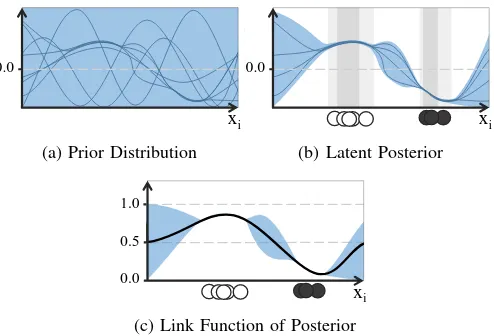
Fig. 1. A sample from a GP can be considered to be a sample of an infinite dimensional Gaussian distribution of candidate functions. Putting a prior on this distribution, restricts it to likely explanations, visualized as blue lines in Figure 1a. The available functions are then further reduced by the presented training data (cf. Figure 1b): In areas where data is sparse, the spread of the functions is higher than in areas with a higher density of training data. Since the range of these functions is unbounded, we apply a link function (cf. Figure 1c) to obtain a probability estimate used for classification. This function then provides the mean (black line) used for prediction and the variance or uncertainty (blue area).

layers, which are referred to ashidden layers. The optimization problem arising when such a deep network is trained is non-convex, hence neural networks are trained using stochastic gradient descent.

E. Support Vector Machines

In contrast to DNNs, Support Vector Machines (SVM) form a convex problem with a unique solution. Given the training data, the goal is to compute a hyperplane separating the data. To achieve a nonlinear decision boundary, a SVM can be kernelized. Since the RBF kernel is similar to the covariance function in GP settings, as we will see now, we investigate RBF SVM in this work. To be able to tell apart SVM and RBF effects, we further also study the linear SVM. Another reason to study SVM is that, as we will see now, GPLVM only yields a latent space, and not a classification output. We thus have to apply a classifier on top, and need the original classifier without the preprocessing as a baseline. When employing SVM on top of GPLVM for classification we pick the kernel according to performance.

F. Gaussian Processes

We consider two applications of Gaussian Processes. First, we use GP directly for classification (GPC). Second, we de-scribe the Gaussian Process Latent Variable Model (GPLVM), which is a mapping from the data to a latent space. Subse-quently, GPLVM is used as a pre-processor to train a SVM classifier.

GP Classification. We introduce here GPC [34] for two classes using the Laplace approximation. The goal is to predict the labels Yt for the test data points Xt accurately. We first

consider regression, and assume that the data is produced by a GP and can be represented using a covariance functionk:

whereKtris the covariance of the training data,Ktof the test data, andKtt between test and training data based onk. The optimum estimate for the posterior mean at given test points, assuming a Gaussian likelihood function is (from [34], page 44, equation 3.21),

which is at the same time the mean of our latent function

f∗. We will not go into details here on how to optimize

the parameters of the covariance function k, but instead move from regression to classification. Since our labels yt are not real valued, but class labels, we ‘squash’ this output using a link function σ(·) such that the output varies only between the two classes (cf. Figure 1). For classification, the optimization can be simplified using the previously stated Laplace approximation. At this point, we want to refer the interested readers to Rasmussen et al. [34].

In addition to the mean, as explained above, we are also able to compute the variance. This allows us to obtain the uncertainty for GPC, and will be used later in this work.

GP Latent Variable Model. GPC learns based on labels. This introduces an implicit bias: we assume for example that the number of labels is finite and fixed. Furthermore, the curse of dimensionality affects classification. This curse affects distance measure on data points. In higher dimensions, the ratio between nearest and furthest point approximates one. All data points are thus uniformly distant, impeding classi-fication: it becomes harder to compute a separating boundary. Consequently, we are interested in finding a lower dimensional representation of our data.

These two issues are taken into account when using GPLVM. Its latent space is a lower-dimensional representation of the data where labels are ignored. A particular property of this latent space is further that it allows for nonlinear con-nections in the feature space to be represented. Additionally, GPLVM models uncertainty estimates, analogously to GPC.

IV. METHODOLOGY

In this section, we first introduce two direct attacks on GP classification. Afterwards, we introduce Latent Space Ap-proximation Networks (LSAN) to approximate GPLVM-based classification. As we will see, these attacks can be leveraged to attack other kernelized methods.

A. Attacks on GPC

As for all classifiers, to produce an adversarial example we need to find the gradient in the output with respect to the input dimensions. We consider the chain of gradients for the output

(5)

wheref∗ andk are the associated latent function and

covari-ance function, respectively.

Note that for our attack, we are only concerned with the rel-ative order of the gradients, we are not interested in the actual values. Unfortunately, σ¯∗ does not vary monotonically with

f∗. For example, consider that if f∗ increases slightly, thus

becoming more positive, the variance of f∗ would increase

massively as well. However, through the link function the mean ofσ¯∗would at the same move downwards, approaching

0.5.

We use the gradient off∗instead a numerical approximation

to σ¯∗. The reasoning is as follows: since we are in a setting

of binary classification, we are only interested in moving the prediction across the 0.5 boundary. No change in variance can cause this, instead a change in the mean off∗is required.

Indeed one can note that the gradient off∗ is an upper bound

on the gradient of σ¯∗. This is due to the fact that the link

function ‘squashes’ the input, however preserving the changes. The fastest we can get from one probability thresholdptto its opposite 1−pt is when there is no variance. So finding the gradient off∗ is sufficient.

Let us first rewrite the expected value off∗ in Equation (3)

given a single test point x∗

:

From here, we can easily move on to the first part of the gradient,

∂f∗

∂k =K

−1

tr ytr (6)

where the terms are both constant w.r.t. the test inputx∗

. The gradient of the kernel w.r.t. the inputs depends on the particular kernel that is applied. In our case, for the RBF kernel, between training pointx∈Xtr and test pointx∗, the gradient can be

where xi and x∗i each denote feature or position i of the corresponding vector or data point and l denotes the length-scale parameter of the kernel. Using the assumption above the gradient of the output σ¯ with respect to the inputs is proportional to the product of Equation (6) and Equation (7). Finally, we introduce the attacks, conceptually related to FGSM and JSMA. The first one introduces a global change based on the sign of the gradients (of a single sample xand the classifierf∗) and someǫ. We depict it in Algorithm 1 and,

due to its similarity with FGSM we call it GPFGS. For both attacks we assume the kernel to be RBF (and thus drop the explicit notation of the kernel gradients). We also compute the gradient as the product of Equation (6) and Equation (7) in both algorithms.

In Algorithm 2 we compute the gradients and add or remove a feature depending on the strongest gradient, analogous to JSMA. Consequently, we call this attack GPJM. In this algorithm, we keep track of the modified features, to avoid

Algorithm 1Given an input samplexand the latent function

f∗, we compute an adversarial example, x ∗

using GPFGS.ǫ

denotes the perturbation introduced for each feature.

Require: x,f∗,ǫ

1: x∗←x∗+ǫ×sign(∇f∗)

2: return x∗

Algorithm 2Given an input samplexand the latent function

f∗, we compute an adversarial example, x ∗

using GPJM. t

denotes the maximal number of features we are allowed to change.

changing a feature twice. We also allow changes in both directions of the gradients, as visible in line10. We iteratively change features until a sample is misclassified, or too many features are changed (more thant).

B. Attacks on GPLVM using Latent Space Approximation Networks

The GPLVM mapping is, similar to kernels, hard to invert. The change in the original data for a corresponding change in latent space is usually hard to determine. We thus try to approximate these methods with DNN, which are easier to invert: there is a wide range of known attacks. The challenge is therefore to produce a substituteLatent Space Approximation Network(LSAN), which is as similar as possible to the original latent space kernel.

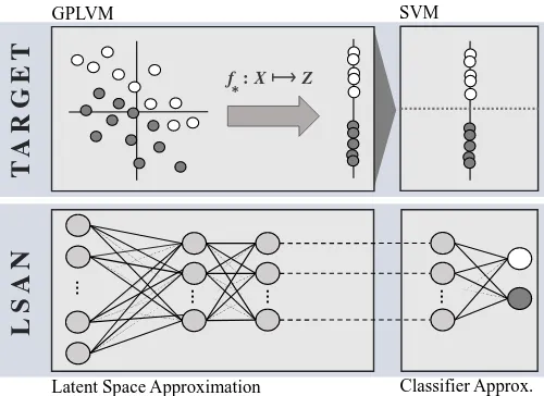
The rough idea is depicted in Figure 2. We approximate the latent space and the classifier by using a DNN. To achieve this, we train the second last layer to mimic the latent space, and treat the last layer as a linear classifier (trained on the latent space as input). If this classifier happens to be nonlinear, we add another intermediate layer to achieve nonlinearity. To apply the known attacks for neural networks, we combine the two parts that are trained separately. As visible in Figure 2, we do this by feeding the output of the latent network directly to the classifier network.

(6)

GPLVM SVM

Fig. 2. The intuition of LSAN. The first network is trained on a latent space, the second to classify input from this latent space. After training, the two networks are combined and yield one DNN classifier.

hence train the output layer of the latent space on the kernel matrix given some fixed points from the dataset. More pre-cisely, the output neurons1. . . nare trained on the particular distance of some data points 1. . . nselected from Xtr.

We can then proceed by using any of the DNN-specific attacks on the LSAN to produce adversarial examples for the original classifiers.

V. EXPERIMENTALSETUP

Before we evaluate the research questions posed in Sec-tion II, we briefly describe the setting of our evaluaSec-tion. We start with the datasets on which the different ML models where evaluated, and move then to the ML models used and their respective implementations2_{. Before diving into the evaluation,} we also briefly comment on convergence and accuracies of all models.

A. Data

We seek to evaluate adversarial examples in two security contexts: Malware classification and Spam detection. In addi-tion to this, we want to evaluate all mechanisms in a commonly used ML benchmark for classification tasks. We carefully selected these datasets to account for the diversity in data types ML models face across different application domains: individual data features may contain binary (e.g. static code features), integer (e.g. pixel values) or real-valued (e.g. fre-quencies) data. Whole datasets may contain widely different amounts of features and with different feature sparsity.

Hidost. Our Malware dataset consists of the PDF Malware data of the Hidost Toolset project [41] The dataset is composed of 439,563 PDF Malware samples, of which 407,037 are labeled as benign and32,567as malicious. Datapoints consist of 1223 binary features and individual feature vectors are

2_{The code, and thus any further details, can be accessed by contacting the} authors

likely to be sparse. We split it in 95% training and 5%. This still leaves us with more than 20,000 test data points to craft adversarial examples, where many attacks are very time consuming to compute.

Spam. The second security-relevant dataset is an email Spam dataset [23]. It contains 4,601 samples. Each sample captures 57 features, of which 54 are continuous and rep-resent word frequencies or character frequencies. The three remaining integer features contain capital run length infor-mation. This dataset is slightly imbalanced: roughly 40% of the samples are classified as Spam, the remainder as benign emails. We split this dataset randomly and use 30% as test data.

MNIST. Finally, we use the MNIST benchmark dataset [22] to select two additional, binary task sub-datasets. It consist of roughly 60,000, 28×28 pixels, black and white images of handwritten single digits. There are 50,000 training and

10,000 test samples, for each of the ten classes roughly the same number. We select two binary tasks: 1 versus 9 and 3

versus 8 (denoted as MNIST91 and MNIST38 respectively). We do this in an effort to study two different tasks on the same underlying data representation, i.e. the same number and range of features, yet with different distributions to learn.

B. Models

We investigate transferability across multiple ML models derived by different algorithms. In some cases, dataset-specific requirements have to be met for classification to succeed.

GPLVM. We train GPLVM generally using 6 latent di-mensions with the exception of the Spam dataset, where more dimensions (32) are needed for good performance. We further use SVM on top of GPLVM to produce the classification results, a linear SVM for the MNIST91 tasks and an RBF-kernel SVM for all other tasks.

LSAN. We distinguish between LSAN approximating GPLVM (GPDNN), linear SVM (linDNN) and RBF SVM (rbfDNN). All of them contain two hidden layers with half as many neurons as the datasets’ respective features. The layer trained on latent space encompasses 30neurons for the SVM networks and 6 neurons for GPDNN, except for the Spam dataset, where we model32 latent variables. From this latent space, we train a single layer for classification, with the exception in GPDNN in the cases where an RBFSVM is trained on top: here we add a hidden layer of2 neurons.

DNN. Our simple DNN accomodates two hidden layers, each containing half as many neurons as the dataset has features, and ReLU activation functions. For the transferability experiments, the DNN has the same architecture as GPDNN.

SVM. We study a linear SVM and a SVM with an RBF kernel. They are optimized using squared hinge loss. We further set the penalty term to1.0. For the RBF kernel, theγ

(7)

C. Implementation and third party libraries

We implement our experiments in Python using the follow-ing specialized libraries: Tensorflow [1] for DNNs, Scipy [18] for SVM and GPy [21] for GPLVM and GPC. We rely on the implementation of the JSMA and FGSM attack from the library Cleverhans version 1.0.0 [12]. We use the code pro-vided by Carlini and Wagner for their attacks3_{. We implement} the linear SVM attack (introduced in [31]) and the GPattacks (based on GPy) ourselves.

D. Accuracy and Convergence of Target Models

Before we start investigating the actual transferability task and the adversarial example crafting, we want to comment on the achieved accuracies on the previously defined datasets. Since we encountered some difficulty training the LSANs, we comment on this as well.

Convergence. LSAN networks need to be trained for7000

iterations, much longer than a conventional DNN. Also its parameters, such as the initial weights, learning rate and bias initialization need to be carefully selected to have the two networks converge.

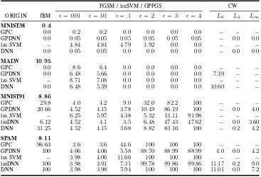
For RBF-DNN, the LSAN approximating RBF-kernel SVMs, we could find no initial parameters to guarantee con-vergence globally. The same holds for the LSAN and a linear kernel on MNIST38 and the Malware data. In two settings, RBF kernel on MNIST91 and linear kernel on MNIST38, we could not find parameters working with two different random seeds (one for white box or direct crafting, one for evaluation in grey box). We thus excluded those networks from the experiments, and marked them in Table I.

Accuracy. The test accuracies of all classifiers are depicted in Table I. We only want to compare ML models which achieve similar accuracies, as not doing so might influence the results in a unpredictable manner. In cases where specific models fail to achieve similar accuracy we exclude the outliers.

For the Spam dataset, the highest accuracy is achieved by DNN (94.2%), other algorithms (GPDNN, GPLVM,GPC, linSVM) vary between 90.1% and 92.7%. On the Malware dataset, all classifiers perform better than 99.2%, where LSANs trained on kernels do not converge. GPDNN achieves the worst accuracy with98.2%. On MNIST91, we also observe all algorithms to perform better than99.2%, with the exception of the LSAN trained on a linear kernel (only 98.9). For MNIST38, the range of accuracies of the resulting classifiers is more diverse. Most classifiers (DNN, GPLVM, GPC and RBFSVM) achieve 97.4% to 98.6%. Linear SVM achieves

96.8%, GPDNN and GPC94.4%.

We exclude all models with low baseline performance, such as rbfDNN (all settings) and RBF SVM on Spam. LinDNN is excluded on all datasets except MNIST91, where however we use it for crafting on the Spam data.

3_{Retrieved from https://github.com/carlini/nn robust attacks, July 2017.}

TABLE I

In this section, we answer all posed research questions given the previously introduced setting. We start with white box setting to provide more background, and then move towards the grey box setting.

In the white box setting, we aim at answering the first RQ. This question, RQ 1, inquires whether we are able to craft adversarial examples on GPC in a white box setting.

We then turn to the grey box setting. Here, we start answering the questions concerning LSAN, RQ 4–RQ 6. We then describe our results concerning GPC and transferability to and from GPC, thus RQ 2 and RQ 3. Finally, we focus on the uncertainty estimates of GP models, and deal with RQ 7 and RQ 8.

A. White Box

Before we start evaluating the experiments, we briefly want to remark on the attacks used on each dataset. In Section III-C we argued which norms are feasible for which data. Since we propose new attacks, however, we ignore these restrictions for the newly introduced attacks to evaluate them without any preconceived bias regarding their usefulness. We also kept other attacks that are not too time consuming in computation, e.g. FGSM, as a comparison.

For each attack, we briefly state how many adversarial examples could be computed using the attack on the benign test data. Additionally, we investigate there average amount of perturbation necessary for misclassification. This measurement refers to either the perturbation computed by the attack (as JSMA, GPJM,Lx) or the perturbation introduced globally (ǫ, for FGSM, GPFGS and the attack on linear SVMs).

(8)

TABLE II

PERCENTAGE OF CORRECTLY CLASSIFIED ADVERSARIAL EXAMPLES

CRAFTED BYJBM (JSMA,GPJM)ANDCWRESPECTIVELY. XDENOTES

MODELS EXCLUDED FROM EVALUATION.

AVERAGE PERCENTAGE OF FEATURES MODIFIED FOR SUCCESSFUL

ADERVSARIALEXAMPLES. JBMDENOTESJSMAANDGPJM,Lx

CARLINIWAGNER EXAMPLES. ALL NUMBERS OBSERVED IN A WHITE BOX SETTING.

On the Malware dataset, JSMA is not able to produce an adversarial example in around 1% of the test samples. On the same dataset, we also observe that LSAN (approximating GPLVM) need higher amount of perturbation to cause mis-classification. On the Spam dataset, we can craft adversarial examples for every test point. The degree of perturbation introduced for fooling DNN and LSAN (GPDNN) is almost the same (3.79 for DNN,3.62for LSAN).

FGSM. On all datasets, we observe that the decrease in accuracy with increasing ǫis much more pronounced on the DNN than on LSAN. This discrepancy is the most noticeable in the Spam dataset, where the accuracy drastically declines for DNN from93.8% whenǫ= 0.001to6.3% whenǫ= 0.4. For LSAN (GPDNN), the accuracy falls from90.1% to22.7% in the same interval. We suspect that this disparity is due to gradient masking and should not be interpreted as LSAN being more robust. When investigating the performance of LSAN in the grey-box setting later on, we will also see no particular evidence for improved robustness.

CW/Lx. Due to the long runtime of these attacks, we crafted a set of500examples for each combination of attacks, classifiers and datasets. Across all datasets, we observe that the algorithms succeed in crafting adversarial examples for every test sample. We also measure the perturbations and depict them in Table III.

SVM-attack. Given the results in Table IV, we observe the strongest effect with examples crafted using the smallest

ǫ−0.001for all datasets. Also for all datasets, the accuracy in the worst case of this attack is roughly the same as a random guess. Compared to the other attacks, this attack is not very effective.

TABLE IV

PERCENTAGE OF CORRECTLY CLASSIFIED ADVERSARIAL EXAMPLES

CRAFTED ON LINEARSVM/DNN FGSM,ORGPFGSIN A WHITE BOX

SETTING.

GPJM and GPFGS. Similar to FGSM, a strongerǫleads to lower accuracy on the crafted adversarial examples. At the same time, there is often a point (ǫ= 0.2 for Spam,ǫ= 0.2

for MNIST91, ǫ = 0.1 for MNIST38), where the accuracy remains almost constant. We then observe no further decrease in accuracy on crafted examples. For GPJM, we observe mixed results, where MNIST91 can be fooled completely. For other datasets, accuracy decreases to28.8% (Spam) and69% (MNIST38).

For both GP attacks it is necessary to invert the kernel matrix. This matrix very sparse for the Malware dataset, and the computation fails. We therefore use a pseudo-inverse to compute the attack. We still observe only a very moderate degree of success: only27% of crafted examples are misclas-sified. We still answer RQ 1 positively—we are able to craft adversarial examples for GPC.

B. Transferability

We now investigate the transferability of the attacks de-scribed in the previous section. We start by investigating the capabilities of LSAN in approximating their counterparts. We then investigate GPC and transferability of the attack derived for, before turning to uncertainty estimates as a defense. For the interested reader, we provide the detailed results to all experiments in the Appendix, and use mainly meta statistics to ease understanding.

C. LSAN: Results of RQ 4–RQ 6

We start by investigating whether LSAN enables attacks on models that use GPLVM latent space representations or kernels in general.

(9)

Table I. When approximating GPLVM, we observe similar accuracies on MNIST91 (LSAN 99.2%, GPLVM 99.34%) and Spam (91.2% versus 91.8% originally). On Malware, LSAN is slightly better than the original by 0.3%. However, on MNIST38, it performs worse by more than three percent. In summary, all these approaches perform much better than random choice, and we thus answer RQ 4 positively. We will now investigate the efficiency when computing attacks on LSAN.

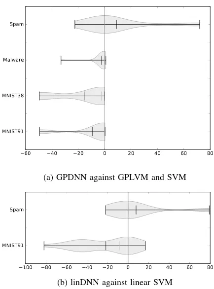
RQ 5. To evaluate this question, we compare the accuracy of the targeted algorithm on different kinds of adversarial examples. In particular, we compare these accuracies on the at-tacks computed on LSAN with all other grey box atat-tacks (like DNN, linear SVM, GPC, and so on). More specifically, we subtract the accuracy on LSAN examples from the accuracy of all other related attacks4_{. We then plot the distribution of these} differences. If the majority of differences is positive, accuracy on adversarial examples computed on LSAN is higher (and thus the LSAN attack performs worse). We depict the results in Figure 3. Ideally, the accuracy of LSAN attacks should be lower, and consequently, the distributions in Figure 3 would be shifted towards the right-hand side.

We consider two settings: one for GPLVM and one for linear SVMs. We start with the results for GPLVM and SVM, aproximated by GPDNN, shown in Figure 3a. For Malware and MNIST91 tasks, we observe that the differences are closely distributed around around zero from the left side. We also observe some outliers, e.g. for Malware we observe the GPJM to be much more effective than other techniques. The accuracy is roughly 61% as compared to over 90% for JSMA on GPDNN. On MNIST91, the linear SVM attack is more effective (reducing accuracy to 50% instead of more than 90%). For MNIST38, we observe that other attacks are more effective. For the Spam data, we observe large variance, indicating that no clear trend towards effectiveness for any particular technique exists. Yet, some positive outliers indicate that GPDNN are more effective than other attacks. This is mainly due to the bad performance of the linear SVM attack (accuracy >90%) and GPJM (55% accuracy, other Jacobian attacks are <20%) on this dataset, however.

We will now investigate the second setting, in particular, the approximation of a linear SVM by LSAN linDNN. We are left with two settings, MNIST91 and Spam, due to convergence. For MNIST91, data is distributed mostly towards the left-hand side, with strong variance, i.e. we conclude other attacks are more effective than LSAN. For Spam, we observe a more centralized distribution, with similar outliers due as observed for GPDNN.

Globally, we do observe however that all medians (gray) are close to 0, i.e. the attacks perform equally.

Given the previous results, we conclude that adversarial examples crafted on LSAN are as effective as other state-of-the-art algorithms in misleading the approximated technique. 4_{We subtract GPDNN FGSM}_ǫ_{= 0}_.₁_{from DNN FGSM}_ǫ_{= 0}_.₁_{, GPFGS}

ǫ= 0.1_{, linear SVM}ǫ= 0.1_{. For Jacobian methods, we subtract GPDNN}

JSMA from DNN JSMA, GPC GPJM, and so on.

60 40 20 0 20 40 60 80

MNIST91 MNIST38 Malware Spam

(a) GPDNN against GPLVM and SVM

100 80 60 40 20 0 20 40 60 80 MNIST91

Spam

(b) linDNN against linear SVM

Fig. 3. EvaluatingRQ 5. We compare the performance of approximated algorithm when classifying adversarial examples crafted on LSAN and other methods. We plot the distribution of differences in accuracy for LSAN exam-ples and examexam-ples from other models. On the right hand side, misclassifcation is higher for LSAN (good). On the left hand side missclassfication is better for other attacks (bad). We also plot mean (black) and median (gray).

We thus answer RQ 5 negatively. A natural question at this point is whether LSAN differs at all from a normal DNN, i.e. whether the process of training a LSAN to approximate a substitute network produces a different result than training the DNN on the unprocessed data in the first place.

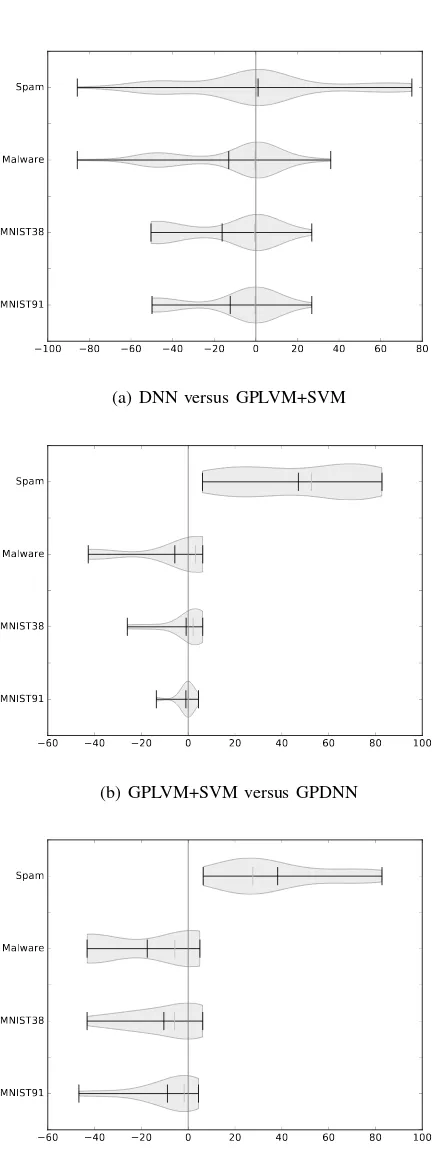
RQ 6. To evaluate this RQ, we rerun the evaluation on adversarial examples with a DNN that has the exact same architecture as the GPDNN. The DNN used in the grey box setting has the same architecture as the GPDNN. For the benign data where both are trained on, we already observed small differences in accuracy described in the previous section. While the networks are trained on benign data, we are interested in their behavior on adversarial examples. We thus compare the difference between the accuracies for all types adversarial examples. Afterwards, we analyze the distribution of the deltas. The results for the four datasets and all three settings are depicted in Figure 4.

(10)

100 80 60 40 20 0 20 40 60 80 MNIST91

MNIST38 Malware Spam

(a) DNN versus GPLVM+SVM

60 40 20 0 20 40 60 80 100

(b) GPLVM+SVM versus GPDNN

60 40 20 0 20 40 60 80 100

(c) DNN versus GPDNN

Fig. 4. EvaluatingRQ 6. We compare the accuracies on adversarial examples of a GPDNN, DNN and GPLVM + SVM on adversarial exmples. To obtain the distributions, we subtract accuracy from the second model from the first model for an attackafor all attacks. Hence on the right hand side, the first model has higher accuracy. On the left hand side, second model performs with higher accuracy. We also plot mean (black) and median (gray) values.

case still larger than 20percentage points. Given the median is always around0, we conclude that although in most cases similar, there can be large differences in the behavior.

b) We now compare GPLVM+SVM and GPDNN, e.g. the latent space classifier and its corresponding LSAN. The results are shown in Figure 4b. We observe that for all datasets except Spam, the distribution are dense around0, e.g. in many cases where the output is very similar. Furthermore, the overall variance is small. There are some cases, however, where GPDNN performs with lower accuracy than GPLVM+SVM: On Spam data, the distribution is far away from0and centered at around50percentage points better. It is also rather uniform. We conclude that GPDNN approximates GPLVM+SVM rather closely on MNIST and the Malware dataset.

c)Finally, we investigate the differences between an LSAN and a DNN, visible in Figure 4c. We observe that for all datasets except Spam, the distribution are heavy around0, e.g. there are many cases where the output is very similar. These findings are, however, not as pronounced as in the previous case. This is due to the higher variance caused by larger differences in the accuracy. For Spam, we observe GPDNN to consistently performs better than DNN. On the other dataset, there are some attacks where GPDNN is slightly better, however also some (MNIST) or many (Malware) settings where GPDNN performs much worse. In general, we observe differences of up to 50 (MNIST, Malware) or >80 (Spam) percentage points.

Given the differences in classification for this range of attacks, we answer all parts of RQ 6 positively. There must be a difference in the inner representations to cause these differences in behavior. We also observe that LSAN is able to approximate the targeted technique. We now conclude our work on LSAN and move on to our attacks on GPC.

D. GPC: Results of RQ 2 and RQ 3

To investigate the transferability concerning GP, we con-sider two perspectives: First, RQ 2, we investigate whether adversarial examples crafted on GPC are misclassified by other algorithms. Second, RQ 3, we question whether adversarial ex-amples crafted on other algorithms are misclassified by GPC. We analyze both perspectives by analyzing the accuracies of both approaches on adversarial examples.

RQ 2. To evaluate this hypothesis, we compare the change in percentage of accuracy for all algorithms except GPC on benign test data and adversarial examples computed on GPC by GPJM and GPFGS 5). We subtract the accuracy on these adversarial examples from the accuracy of benign test data and then plot the distribution of the deltas in Figure 5.

For all datasets, we conclude that the adversarial examples crafted for GPC are also misclassified by other algorithms. We further observe the average reduction is 20percentage points for MNIST. For the Malware data, the average decrease is slightly higher, and around 27%. With > 40%, the average

(11)

0 20 40 60 80 MNIST91

MNIST38 Malware Spam

Fig. 5. EvaluatingRQ 2. We compare the reduction in accuracy of non GPC models to adversarial examples crafted on GPC by substracting the accuracy on examples crafted on GPFGS and GPJM from the accuracy on benign test data. We further plot the distribution of these differences. On the right hand side (of0_{) accuracy decreases. We also plot mean (black) and median (gray).}

weil

decrease is largest in the Spam data. In some cases, we observe a small increases in accuracy, this is the case for Spam and MNIST data. These increases in accuracy are generally observed for GPFGS for small values ofǫ, such as 0.001and

0.01. Analogously to FGSM, a largerǫimplies higher rate of misclassification.

RQ 3. We will now investigate the opposite direction, e.g. transferability from adversarial examples crafted on other models on GPC. To answer this question, we subtract the accuracy on some adversarial examples (all attacks crafted on non-GPC models) from the accuracy on benign test data. We plot the distribution of these differences in Figure 6.

We observe for all datasets, attacks and algorithms we crafted on that they also mislead GPC. The average decrease is, compared to the previous findings, however smaller. Consider an average reduction of 30% versus > 40% on the Mal-ware data, and roughly 15% versus 20% on MNIST91. For MNIST38, the results are similar on avergage. For Malware, we observe almost no reductions; however we in general observe (also for other models) that attacks have low trans-ferability.

We further observe some cases where accuracy increases for adversarial examples on GPC. We observe this on Spam and MNIST38. On the Spam data, this is caused by the linear SVM attack. This attack is classified (by all models) correctly in all cases. On MNIST38, the cases where accuracy increases are FGSM examples with lowǫ.

From the previous finding, we conclude that transferability holds in both directions for GPC. This refers to both adversar-ial examples crafted on other techniques exported to GPC and vice versa. We thus answer both RQ 2 and RQ 3 positively. Given this result, we confirm the threat of adversarial examples also for GP. On the other hand, there is a crucial difference

20 0 20 40 60 80 100

Fig. 6. EvaluatingRQ 3. We compare the accuracy of GPC on adversarial examples (of all models, except GPC). In particular, we subtract the accuracy on adversarial examples from the accuracy on benign test data. We plot the distribution of these values. Hence, values>0_{show an decrease of accuracy,}

values>0_{and increase of accuracy. We also plot mean (black) and median}

(gray).

between a DNN and any GP; uncertainty. We now turn to this property of GP and investigate whether it is able to alleviate the effect of adversarial examples.

E. Uncertainty: Results of RQ 7 and RQ 8

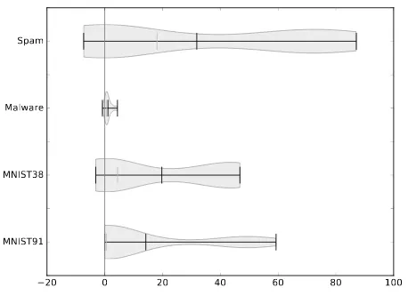
Intuitively, the variance of a prediction is low in areas where training data was observed6_{. Accordingly, we might} expect the variance to be larger in the vicinity of adversarial examples. Adversarial examples are likely to lie in regions away from training data: In high-dimensions the training data is likely contained on a low-dimensional manifold which is not orthogonal to the decision boundary. The creation of an adversarial example usually involves moving towards the boundary along a short path. However this process usually moves it away from the regions of training data, and thus towards areas with few data points, leading to increasing classification uncertainty. This hypothesis is consistent with the empirically validated assumption that adversarial examples stem from a distribution statistically separate from the training data [13]. Hence, we have investigate the variance reported in the two GP approaches. In particular, we compare the mean variance across all adversarial examples and the mean variance across all benign data points. In the case of GPC, we also investigate the average absolute value of the latent function. The intuition is that the behavior of this latent function is as well different in areas where no data was observed. The GPLVM, as an unsupervised ML method, does not use class labels in its initial training and its latent function is therefore interpreted differently. Here the value of the latent function is treated as the actual position in the transformed data space. We will start with GPC (RQ 7).

(12)

TABLE V

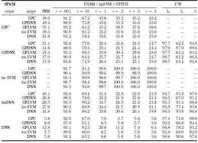
REJECTED DATA OUTSIDE A95_%CONFICENDE INTERVAL IN PERCENT: BENIGN DATA(BOLD)AND ADVERSARIAL EXAMPLED CRAFTED ON MODEL

ORIGIN

FGSM / linSVM / GPFGS CW

ORIGIN JBM ǫ=.001 ǫ=.01 ǫ=.1 ǫ=.2 ǫ=.3 ǫ=.4 L0 L2 L∞

MNIST38 0.4

GPC 0.0 0.2 0.2 0.0 0.0 0.0 0.0 ₋ ₋ ₋

GPDNN 0.0 0.05 0.05 0.05 0.05 0.05 0.05 ₋ 0.0 0.0

lin SVM − 4.84 4.84 4.79 1.92 0.0 0.0 ₋ ₋ ₋

DNN 0.0 0.05 0.05 0.0 0.0 0.0 0.0 ₋ 0.0 0.0

MALW 10.95

GPC 0.0 8.6 6.4 0.0 0.0 0.0 0.0 ₋ ₋ ₋

GPDNN 0.0 6.48 5.66 0.0 0.0 0.0 0.0 7.39 ₋ ₋

lin SVM − 8.71 7.08 0.0 0.0 0.0 0.0 − − −

DNN 0.0 6.48 5.39 0.0 0.0 0.0 0.0 10.60 ₋ ₋

MNIST91 8.86

GPC 29.8 4.0 4.2 9.0 32.0 82.2 100 ₋ ₋ ₋

GPDNN 20.66 4.52 4.15 3.78 10.49 86.19 100 ₋ 0.0 4.0

lin SVM − 6.25 5.97 4.38 5.32 13.11 91.98 − − −

linDNN 6.12 4.52 4.1 3.5 6.48 47.43 47.62 ₋ 0.0 3.60

DNN 31.25 4.52 4.15 3.68 8.82 83.16 100 ₋ 0.2 4.2

SPAM 8.11

GPC 96.63 3.6 3.6 44.6 100 100 100 ₋ ₋ ₋

GPDNN 100 4.06 4.06 5.58 88.70 88.99 88.99 4.0 0.0 4.2

lin SVM − 3.98 4.06 11.66 100 100 100 − − −

linDNN 100 3.98 3.91 7.31 99.78 99.86 99.86 11.17 0.2 9.0

DNN 100 3.98 3.98 5.94 100 100 100 11.01 0.0 7.2

TABLE VI

AVERAGE VARIANCE OFGPC’S LATENT FUNCTION FOR BENIGN DATA(BOLD)AND ADVERSARIAL EXAMPLES CRAFTED ON MODELORIGIN.

MNIST91 6.382

GPC 11.2881 6.6112 6.6309 7.9870 11.9395 18.3882 27.2005 ₋ ₋ ₋

GPDNN 10.0864 6.3756 6.3226 6.8299 9.9377 15.5973 23.6065 ₋ 3.5384 6.1729

lin SVM − 6.5400 6.4951 6.5498 8.1024 11.1595 15.6267 − − −

linDNN 9.3149 6.3751 6.3152 6.2002 7.2703 9.5647 13.0087 ₋ 3.3542 6.3026

DNN 11.0323 6.3755 6.3225 6.8148 9.8171 15.2891 23.0491 ₋ 3.3890 6.4451

SPAM 6.1651

GPC 103.1185 6.3407 6.5151 38.4048 131.4167 199.3153 215.8200 ₋ ₋ ₋

GPDNN 132.7886 6.6645 6.5974 17.2383 57.2994 116.3130 162.1923 6.6377 0.6579 7.1669

lin SVM − 6.6432 6.8533 25.3305 81.3637 151.2960 196.8120 − − −

linDNN 125.1362 6.6596 6.5697 19.3221 66.0221 131.8758 182.6009 8.4672 0.7560 6.1990

DNN 129.9440 6.6452 6.4237 17.1022 60.0533 125.3152 179.3707 7.3519 0.6059 6.7201

RQ 7. The averaged variance values for the tested cases are shown in Table VI. We can immediately observe that the different type of attacks have different degrees of impact on the variance. The most noticeable changes are related to methods that introduce global changes. The larger these changes, the larger the increase in variance of GPC. The variance also strongly increases for all Jacobian based methods. Interest-ingly, we see a decrease in variance forL2and small increases

for the other attack metrics in adversarial examples crafted by the Carlini-Wagner (CW) algorithms.

We also observe differences when monitoring the averaged absolute latent function. The detailed results for this experi-ment are shown in the Appendix.

We thus investigate a straight forward defense, which is

computing the 95% confidence interval of the data and re-jecting all data points that are outside this interval. Here, we use both the latent variance and latent mean. We present our results in Table V. We observe this simple step to be very successful on the Spam data (except on the Lx attacks). On MNIST91 we observe mixed results. On MNIST38 and the Malware data the approach does not work well. An additional observation is that on the two datasets where the defense works well, LSAN examples are in many cases harder to detect than other adversarial examples.

(13)

TABLE VII

AVERAGE VARIANCE OFGPLVMPREDICTIONS FOR BENIGN DATA(BOLD)AND ADVERSARIAL EXAMPLES. ADVERSARIAL EXAMPLES CRAFTED BY

ALGORITHMORIGIN

SPAM 2.3e−06

GPC 0.0001 2.4e−06 ₂_.₄_e−06 ₄_.₅_e−06 ₁_.₆_e−05 ₅_.₃_e−05 ₀_.₀₀₀₁

− − −

GPDNN 8.4e−06 ₂_.₄_e−06 ₂_.₄_e−06 ₃_.₇_e−06 ₈_.₈_e−06 ₂_.₂_e−05 ₅_.₂_e−05 ₂_.₆_e−06 ₁_.₄_e−06 ₂_.₇_e−06 lin SVM − 2.3e−06 ₂_.₃_e−06 ₃_.₂_e−06 ₆_.₂_e−06 ₁_.₃_e−05 ₂_.₇_e−05

− − −

linDNN 5.6e−05 ₂_.₄_e−06 ₂_.₅_e−06 ₄_.₅_e−06 ₁_.₂_e−05 ₃_.₀_e−05 ₇_.₀_e−05 ₂_.₉_e−06 ₁_.₅_e−06 ₂_.₃_e−06 DNN 1.4e−05 ₂_.₄_e−06 ₂_.₄_e−06 ₃_.₆_e−06 ₈_.₆_e−06 ₂_.₁_e−05 ₄_.₉_e−05 ₂_.₄_e−06 ₁_.₄_e−06 ₃_.₀_e−06

MNIST91 0.0083

GPC 0.0083 0.0083 0.0083 0.0083 0.0083 0.0083 0.0083 ₋ ₋ ₋

GPDNN 0.0083 0.0083 0.0083 0.0084 0.0077 0.0065 0.0058 ₋ 0.0081 0.0083

lin SVM − 0.0083 0.0083 0.0083 0.0083 0.0083 0.0083 − − −

linDNN 0.0083 0.0083 0.0083 0.0083 0.0080 0.0077 0.0076 ₋ 0.0081 0.0083

DNN 0.0085 0.0083 0.0083 0.0085 0.0078 0.0066 0.0060 ₋ 0.0081 0.0083

MALW 0.0682

GPC 0.0889 0.0714 0.0712 0.0760 0.0882 0.1102 0.1160 ₋ ₋ ₋

GPDNN 0.0731 0.0736 0.0735 0.0740 0.0775 0.0879 0.2297 0.0892 ₋ ₋

lin SVM − 0.0632 0.0640 0.1000 0.0955 0.0799 0.2779 − − −

DNN 0.0784 0.0737 0.0736 0.0748 0.0738 0.0753 0.1035 0.0553 ₋ ₋

MNIST38 0.0208

GPC 0.0208 0.0208 0.0208 0.0208 0.0208 0.0208 0.0208 ₋ ₋ ₋

GPDNN 0.0208 0.0208 0.0208 0.0207 0.0207 0.0207 0.0207 ₋ 0.0207 0.0208

lin SVM − 0.0208 0.0208 0.0208 0.0208 0.0208 0.0208 − − −

DNN 0.0208 0.0208 0.0208 0.0207 0.0207 0.0207 0.0207 ₋ 0.0207 0.0208

defense. It will be future work to investigate how to improve this by selecting other thresholds. Further we can influence the parameters learned for the covariance function. In our case, this function is similar to the RBF kernel, for which many security properties are known already [37].

Therefore, these measures mitigate some of the threat ad-versarial examples pose. We thus answer RQ 7 positively.

RQ 8. We show the variances of GPLVM for all kinds of adversarial examples in Table VII. For both MNIST tasks, we observe changes of +0.0001 or +0.0005 in the variance, if there are changes at all. For the Malware and Spam data, we do observe some changes: on the Spam data, the variance is an order of magnitude less. On the Malware data, variance shifts from0.068 to0.074 or0.08.

As the degree of the differences is relatively insignificant, we suspect the variance provided in the predictions of GPLVM is not sufficiently informative about whether a data point is an adversarial example. We therefore cannot give a conclusive answer to RQ 8. Nevertheless, we might be able to modify GPLVM’s kernel to cause greater sensitivity to adversarial input. For example, shortening its lengthscale might force the variance to increase more quickly when moving away from training data locations. Investigating and determining the optimal hyper-parameters to alleviate the threat of adversarial examples for GPLVM is left as future work.

VII. RELATEDWORK

Transferability has been investigated in the context of adversarial examples has been brought up by Papernot et al. [31]. Rosza et al.[36] study transferability for different

deep neural network architectures, whereas Liu et al. [24] investigate targeted transferability in particular. Finally Tramer et al. [44] explore transferability by examining the decision boundaries of different classifiers.

In contrast to all these works, we target explicitly security contexts with their binary setting. We further also focus on the usage of kernels and latent space and their effect on transferability.

Other, loosely related works included the work by Biggio et al. [4] and Papernot et al. [31]. Both introduce several attacks, among them attacks for SVM. In our work, we do not target SVM directly, but approximate them to apply common neural network based attacks.

To the best of our knowledge, there is only one approach to connect Gaussian processes to adversarial machine learning by Bradshaw et al. [6]. They do, however, only consider so-called Gaussian Hybrid networks, where the last layer of the neural network is replaced by a Gaussian process, and they evaluate the robustness of hybrid DNNs based only on FGSM and the attack by Carlini and Wagner. In contrast, our work targets Gaussian latent space models and Gaussian Pro-cess classification and studies transferability more extensively, using adversarial examples crafted by more algorithms and across several datasets.

VIII. CONCLUSION

(14)

First, Gaussian Processes are as well vulnerable to ad-versarial examples. We constructed three novel attacks on GPs: Targeting GP classification in a supervised setting, we developed GPFGS and GPJM. Targeting GP Latent Variable models in an unsupervised setting, we proposed LSAN, a novel approach to approximating an arbitrary Latent Space representation.

Second, LSAN adversarial examples exhibit a less notice-able impact on uncertainty estimates while causing a similar amount of missclassifications. Further, LSAN approximate their target latent space models well in terms of behavior.

Third, Adversarial examples produced by state-of-the-art attacks noticeably affect uncertainty estimates in GP classifi-cation. We empirically investigated how adversarial examples affect the uncertainty estimates. In the case of GP classifica-tion, we observed significant changes to the latent function mean values and variance, suggesting that as adversarial examples attempt to cross the classification boundary, they also move towards areas of lower confidence. Interestingly, we also observe that the uncertainty estimates even vary between adversarial examples produced by different algorithms. Finally, we implemented a straight forward defense based on the95% confidence of the latent function of GPC. We observe this simple defense to work reasonably well in two of four datasets. Determining further configuration and effect of parameters learned by GPC is, however, left as future work.

ACKNOWLEDGMENT

This work was supported by the German Federal Ministry of Education and Research (BMBF) through funding for the Center for IT-Security, Privacy and Accountability (CISPA) (FKZ: 16KIS0753). This work has further been supported by the Engineering and Physical Research Council (EPSRC) Research Project EP/N014162/1.

REFERENCES

[1] M. Abadi, P. Barham, J. Chen, Z. Chen, A. Davis, J. Dean, M. Devin, S. Ghemawat, G. Irving, M. Isard, M. Kudlur, J. Levenberg, R. Monga, S. Moore, D. G. Murray, B. Steiner, P. A. Tucker, V. Vasudevan, P. Warden, M. Wicke, Y. Yu, and X. Zheng. Tensorflow: A system for large-scale machine learning. In12th USENIX Symposium on Operating Systems Design and Implementation, OSDI 2016, Savannah, GA, USA, November 2-4, 2016., pages 265–283, 2016.

[2] I. Androutsopoulos, J. Koutsias, K. V. Chandrinos, G. Paliouras, and C. D. Spyropoulos. An evaluation of naive bayesian anti-spam filtering.

arXiv preprint cs/0006013, 2000.

[3] M. Barreno, B. Nelson, A. D. Joseph, and J. D. Tygar. The security of machine learning.Machine Learning, 81(2):121–148, 2010.

[4] B. Biggio, I. Corona, D. Maiorca, B. Nelson, N. Srndic, P. Laskov, G. Giacinto, and F. Roli. Evasion attacks against machine learning at test time. InMachine Learning and Knowledge Discovery in Databases - European Conference, ECML PKDD 2013, Prague, Czech Republic, September 23-27, 2013, Proceedings, Part III, pages 387–402, 2013. [5] B. Biggio, G. Fumera, F. Roli, and L. Didaci. Poisoning adaptive

biometric systems. In Structural, Syntactic, and Statistical Pattern Recognition - Joint IAPR International Workshop, SSPR&SPR 2012, Hiroshima, Japan, November 7-9, 2012. Proceedings, pages 417–425, 2012.

[6] J. Bradshaw, A. G. d. G. Matthews, and Z. Ghahramani. Adversarial Examples, Uncertainty, and Transfer Testing Robustness in Gaussian Process Hybrid Deep Networks.ArXiv e-prints, July 2017.

[7] N. Carlini and D. Wagner. Towards evaluating the robustness of neural networks.CoRR, abs/1608.04644, 2016.

[8] N. Carlini and D. A. Wagner. Adversarial examples are not easily detected: Bypassing ten detection methods. CoRR, abs/1705.07263, 2017.

[9] A. P. Engelbrecht. Using the taylor expansion of multilayer feedforward neural networks. South African Computer Journal, 26:181–189, 2000. [10] C. Farabet, C. Couprie, L. Najman, and Y. LeCun. Scene parsing with

multiscale feature learning, purity trees, and optimal covers. arXiv preprint arXiv:1202.2160, 2012.

[11] I. J. Goodfellow et al. Explaining and harnessing adversarial examples. In Proceedings of the 2015 International Conference on Learning Representations, 2015.

[12] I. J. Goodfellow, N. Papernot, and P. D. McDaniel. cleverhans v0.1: an adversarial machine learning library.CoRR, abs/1610.00768, 2016. [13] K. Grosse, P. Manoharan, N. Papernot, M. Backes, and P. McDaniel.

On the (Statistical) Detection of Adversarial Examples.ArXiv e-prints, Feb. 2017.

[14] K. Grosse, N. Papernot, P. Manoharan, M. Backes, and P. McDaniel. Adversarial perturbations against deep neural networks for malware classification. CoRR, abs/1606.04435, 2016.

[15] Y. Han and B. I. P. Rubinstein. Adequacy of the Gradient-Descent Method for Classifier Evasion Attacks. ArXiv e-prints, Apr. 2017. [16] W. Hu and Y. Tan. Generating Adversarial Malware Examples for

Black-Box Attacks Based on GAN. ArXiv e-prints, Feb. 2017.

[17] X. Huang, M. Kwiatkowska, S. Wang, and M. Wu. Safety verification of deep neural networks. InInternational Conference on Computer Aided Verification, pages 3–29. Springer, 2017.

[18] E. Jones, T. Oliphant, P. Peterson, et al. SciPy: Open source scientific tools for Python, 2001–. [Online; accessed ¡today¿].

[19] G. Katz, C. W. Barrett, D. L. Dill, K. Julian, and M. J. Kochenderfer. Reluplex: An efficient SMT solver for verifying deep neural networks.

CoRR, abs/1702.01135, 2017.

[20] R. Laishram and V. V. Phoha. Curie: A method for protecting SVM classifier from poisoning attack. CoRR, abs/1606.01584, 2016. [21] N. D. Lawrence. Gaussian process latent variable models for

visual-isation of high dimensional data. In Advances in neural information processing systems, pages 329–336, 2004.

[22] Y. Lecun, L. Bottou, Y. Bengio, and P. Haffner. Gradient-based learning applied to document recognition. InProceedings of the IEEE, pages 2278–2324, 1998.

[23] M. Lichman. UCI machine learning repository, 2013.

[24] Y. Liu, X. Chen, C. Liu, and D. Song. Delving into transferable adversarial examples and black-box attacks. CoRR, abs/1611.02770, 2016.

[25] S. M. Loos, G. Irving, C. Szegedy, and C. Kaliszyk. Deep network guided proof search. CoRR, abs/1701.06972, 2017.

[26] D. Lowd and C. Meek. Good word attacks on statistical spam filters. In

CEAS 2005 - Second Conference on Email and Anti-Spam, July 21-22, 2005, Stanford University, California, USA, 2005.

[27] D. Maiorca, I. Corona, and G. Giacinto. Looking at the bag is not enough to find the bomb: an evasion of structural methods for malicious PDF files detection. In8th ACM Symposium on Information, Computer and Communications Security, ASIA CCS ’13, Hangzhou, China May 08 -10, 2013, pages 119–130, 2013.

[28] M. McCoyd and D. Wagner. Spoofing 2D Face Detection: Machines See People Who Aren’t There.ArXiv e-prints, Aug. 2016.

[29] S.-M. Moosavi-Dezfooli, A. Fawzi, and P. Frossard. Deepfool: A simple and accurate method to fool deep neural networks. In The IEEE Conference on Computer Vision and Pattern Recognition (CVPR), June 2016.

[30] N. Narodytska and S. P. Kasiviswanathan. Simple black-box adversarial perturbations for deep networks. CoRR, abs/1612.06299, 2016. [31] N. Papernot, P. McDaniel, and I. J. Goodfellow. Transferability in

ma-chine learning: from phenomena to black-box attacks using adversarial samples.CoRR, abs/1605.07277, 2016.

[32] N. Papernot, P. McDaniel, S. Jha, M. Fredrikson, Z. B. Celik, and A. Swami. The Limitations of Deep Learning in Adversarial Settings. InProceedings of the 1st IEEE European Symposium in Security and Privacy (EuroS&P), 2016.

[33] N. Papernot, P. D. McDaniel, A. Sinha, and M. P. Wellman. Towards the science of security and privacy in machine learning. CoRR, abs/1611.03814, 2016.

(15)

[35] K. Rieck, P. Trinius, C. Willems, and T. Holz. Automatic analysis of malware behavior using machine learning. Journal of Computer Security, 19(4):639–668, 2011.

[36] A. Rozsa, M. G¨unther, and T. E. Boult. Are Accuracy and Robustness Correlated?ArXiv e-prints, Oct. 2016.

[37] P. Russu, A. Demontis, B. Biggio, G. Fumera, and F. Roli. Secure kernel machines against evasion attacks. InAISec@CCS, pages 59–69. ACM, 2016.

[38] J. Saxe and K. Berlin. Deep neural network based malware detection using two dimensional binary program features. In10th International Conference on Malicious and Unwanted Software, MALWARE 2015, Fajardo, PR, USA, October 20-22, 2015, pages 11–20, 2015. [39] R. Sommer and V. Paxson. Outside the closed world: On using machine

learning for network intrusion detection. In2010 IEEE symposium on security and privacy, pages 305–316. IEEE, 2010.

[40] N. Srndic and P. Laskov. Practical evasion of a learning-based classifier: A case study. In2014 IEEE Symposium on Security and Privacy, SP 2014, Berkeley, CA, USA, May 18-21, 2014, pages 197–211, 2014. [41] N. ˇSrndi´c and P. Laskov. Hidost: a static machine-learning-based

detector of malicious files.EURASIP Journal on Information Security, 2016(1):22, Sep 2016.

[42] C. Szegedy, W. Zaremba, I. Sutskever, J. Bruna, D. Erhan, I. Goodfellow, and R. Fergus. Intriguing properties of neural networks. InProceedings of the 2014 International Conference on Learning Representations. Computational and Biological Learning Society, 2014.

[43] C. Szegedy, W. Zaremba, I. Sutskever, J. Bruna, D. Erhan, I. J. Goodfellow, and R. Fergus. Intriguing properties of neural networks.

CoRR, abs/1312.6199, 2013.

[44] F. Tram`er, N. Papernot, I. Goodfellow, D. Boneh, and P. McDaniel. The Space of Transferable Adversarial Examples.ArXiv e-prints, Apr. 2017. [45] F. Tram`er, F. Zhang, A. Juels, M. K. Reiter, and T. Ristenpart. Stealing machine learning models via prediction apis. In25th USENIX Security Symposium, USENIX Security 16, Austin, TX, USA, August 10-12, 2016., pages 601–618, 2016.

[46] P. Vidnerov´a and R. Neruda. Vulnerability of machine learning models to adversarial examples. InProceedings of the 16th ITAT Conference Information Technologies - Applications and Theory, Tatransk´e Matliare, Slovakia, September 15-19, 2016., pages 187–194, 2016.

[47] W. Xu, Y. Qi, and D. Evans. Automatically evading classifiers. In

Proceedings of the 2016 Network and Distributed Systems Symposium, 2016.

(16)

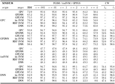
MNIST38 FGSM / linSVM / GPFGS CW

origin target JBM ǫ=.001 ǫ=.01 ǫ=.1 ǫ=.2 ǫ=.3 ǫ=.4 l2 li

GPC 72.9 95.6 95.8 95.6 95.8 84.2 50.4 ₋ ₋

GPDNN 65.2 93.2 93.6 88.8 80.8 74.8 68.6 ₋ ₋

GPLVM 75.5 97.2 97.4 97.2 94.8 93.0 89.6 ₋ ₋

GPC lin SVM 76.8 97.4 96.4 78.0 65.2 58.6 54.8 ₋ ₋

RBF SVM 77.4 98.0 98.0 94.4 87.8 82.2 78.6 ₋ ₋

DNN 81.9 99.2 99.2 95.2 83.2 73.6 65.0 ₋ ₋

GPC 93.8 94.7 94.8 94.7 91.3 66.4 49.0 53.2 94.2

GPDNN 94.2 93.8 93.9 90.8 81.4 68.2 57.9 52.6 94.6

GPLVM 97.7 97.6 97.7 97.7 97.3 95.4 90.3 53.4 98.4

GPDNN lin SVM 92.7 96.9 96.7 86.0 75.4 74.1 73.9 52.8 97.2

RBF SVM 96.9 97.4 97.3 96.8 93.8 88.2 80.0 52.6 97.4

DNN 98.4 98.7 98.7 97.8 94.2 85.7 73.2 52.8 98.6

GPC − 47.7 47.6 47.8 48.4 48.2 49.0 ₋ ₋

GPDNN − 48.5 48.5 49.3 50.9 50.8 48.1 − −

GPLVM − 48.2 48.1 48.2 48.4 48.6 48.6 ₋ ₋

linSVM lin SVM − 48.3 48.5 49.1 49.1 49.1 49.1 − −

RBF SVM − 48.2 48.3 48.5 49.1 49.3 49.2 ₋ ₋

DNN − 48.3 48.3 48.8 48.6 49.3 49.1 − −

GPC 90.8 94.7 94.6 93.1 89.1 64.7 49.1 54.4 95.8

GPDNN 91.0 93.8 93.6 89.0 77.5 61.8 48.5 66.0 93.2

GPLVM 97.3 97.6 97.6 97.0 94.6 87.2 71.6 43.2 98.2

DNN lin SVM 84.9 96.9 95.9 59.0 47.5 44.9 41.3 53.2 96.6

RBF SVM 95.8 97.4 97.1 91.1 68.0 37.8 17.8 59.4 97.2

DNN 97.4 98.7 98.6 91.6 51.8 22.3 8.6 47.4 98.8

TABLE VIII

GRAY BOX EVALUATION ONMNIST38FOR ALL DESCRIBED ATTACKS. PERCENTAGE INDICATED HOW MANY ADVERSARIAL EXAMPLES ARE CORRECTLY CLASSIFIED BT THE MODEL INtarget,WHEN CRAFTED ONoriginUSING THE CORRESPONDING ATTACK. JBMDENOTESJACOBIANBASEDMETHODS,

SUCH ASJSMAONDNNORGPJMFORGPC.−DENOTES THAT AN ATTACK WAS NOT IMPLEMENTED FOR A GIVEN ALGORITHM. METHODS WITH