Nonparametric Shape-restricted Regression
Adityanand Guntuboyina∗ and Bodhisattva Sen†Department of Statistics University of California at Berkeley
423 Evans Hall Berkeley, CA 94720 e-mail:[email protected]
Department of Statistics Columbia University 1255 Amsterdam Avenue
New York, NY 10027 e-mail:[email protected]
Abstract: We consider the problem of nonparametric regression under shape con-straints. The main examples include isotonic regression (with respect to any partial or-der), unimodal/convex regression, additive shape-restricted regression, and constrained single index model. We review some of the theoretical properties of the least squares estimator (LSE) in these problems, emphasizing on the adaptive nature of the LSE. In particular, we study the risk behavior of the LSE, and its pointwise limiting distribu-tion theory, with special emphasis to isotonic regression. We survey various methods for constructing pointwise confidence intervals around these shape-restricted functions. We also briefly discuss the computation of the LSE and indicate some open research problems and future directions.
Keywords and phrases: adaptive risk bounds, bootstrap, Chernoff’s distribution, convex regression, isotonic regression, likelihood ratio test, monotone function, order preserving function estimation, projection on a closed convex set, tangent cone.
1. Introduction
In nonparametric shape-restricted regression the observations{(xi, yi) :i= 1, . . . , n}satisfy
yi =f(xi) +εi, fori= 1, . . . , n, (1)
wherex1, . . . , xnare design points in some space (e.g.,Rd,d≥1),ε1, . . . , εnare unobserved
mean-zero errors, and the real-valued regression function f is unknown but obeys certain known qualitative restrictions like monotonicity, convexity, etc. Let F denote the class of all such regression functions. Letting θ∗ := (f(x1), . . . , f(xn)), Y := (y1, . . . , yn) and
ε:= (ε1, . . . , εn), model (1) may be rewritten as
Y =θ∗+ε, (2)
and the problem is to estimate θ∗ and/orf fromY, subject to the constraints imposed by the properties of F. The constraints on the function classF translate to constraints on θ∗ of the form θ∗ ∈ C, where
C:={(f(x1), . . . , f(xn))∈Rn:f ∈ F} (3) ∗Supported by NSF CAREER Grant DMS-16-54589.
†Supported by NSF Grants DMS-17-12822 and AST-16-14743.
1
is a subset of Rn (in fact, in most cases,C will be a closed convex set). In the following we give some examples of shape-restricted regression.
Example 1.1 (Isotonic regression). Probably the most studied shape-restricted regression problem is that of estimating a monotone (nondecreasing) regression function f when x1 <
. . . < xn are univariate design points. In this case, F is the class of all nondecreasing functions on the interval [x1, xn], and the constraint setC reduces to
I :={(θ1, . . . , θn)∈Rn:θ1 ≤. . .≤θn}, (4)
which is a closed convex cone in Rn (I is defined through n−1 linear constraints). The above problem is typically known as isotonic regression and has a long history in statistics; see e.g., [20, 4, 124].
Example 1.2 (Order preserving regression on a partially ordered set). Isotonic regression can be easily extended to the setup where the covariates take values in a space X with a partial order -1; see e.g., [106, Chapter 1]. A functionf :X →Ris said to be isotonic (or order preserving) with respect to the partial order -if for every pair u, v∈ X,
u-v ⇒ f(u)≤f(v).
For example, suppose that the predictors take values inR2 and the partial order -is defined
as (u1, u2) - (v1, v2) if and only if u1 ≤ v1 and u2 ≤ v2. This partial order leads to a
natural extension of isotonic regression to two-dimensions; see e.g., [67, 105, 26]. One can also consider other partial orders; see e.g., [117,118] and the references therein for isotonic regression with different partial orders. We will introduce and study yet another partial order in Section 6.
Given data from model (1), the goal is to estimate the unknown regression function f :X →Runder the assumption thatf is order preserving (with respect to the partial order
-). The restrictions imposed by the partial order - constrain θ∗ to lie in a closed convex cone C which may be expressed as
{(θ1, . . . , θn)∈Rn:θi ≤θj for everyi, j such that xi -xj}.
Example 1.3 (Convex regression). Suppose that the underlying regression function f : Rd→R (d≥1) is known to be convex, i.e., for everyu, v∈Rd,
f(αu+ (1−α)v)≤αf(u) + (1−α)f(v), for every α∈(0,1). (5)
Convexity appears naturally in many applications; see e.g., [69, 79, 35] and the references therein. The convexity of f constrainsθ∗ to lie in a (polyhedral) convex set C ⊂Rn which, when d= 1 and the xi’s are ordered, reduces to
K:=
(θ1, . . . , θn)∈Rn:
θ2−θ1
x2−x1 ≤
. . .≤ θn−θn−1
xn−xn−1
, (6)
whereas for d≥2 the characterization of C is more complex; see e.g., [109].
1
A partial order is a binary relation-that is reflexive (x-xfor allx∈ X), transitive (u, v, w∈ X, u-v
Observe that when d = 1, convexity is characterized by nondecreasing derivatives (sub-gradients). This observation can be used to generalize convexity to k-monotonicity (k≥1): a real-valued function f is said to be k-monotone if its (k−1)’th derivative is monotone; see e.g., [85, 25]. For equi-spaced design points in R, this restriction constrains θ∗ to lie in the set
{θ∈Rn:∇kθ≥0} where ∇:Rn→Rnis given by ∇(θ) := (θ
2−θ1, θ3−θ2, . . . , θn−θn−1,0)and∇k represents
the k-times composition of ∇. Note that the case k = 1 and k = 2 correspond to isotonic and convex regression, respectively.
Example 1.4 (Unimodal regression). In many applications f, the underlying regression function, is known to be unimodal; see e.g., [45,24] and the references therein. Let Im,1≤ m≤n, denote the convex set of all unimodal vectors (first decreasing and then increasing) with mode at position m, i.e.,
Im :={(θ1, . . . , θn)∈Rn:θ1≥. . .≥θm ≤θm+1≤. . .≤θn}.
Then, the unimodality of f constrainsθ∗ to belong toU :=∪n
m=1Im. Observe that nowU is not a convex set, but a union of n convex cones.
Example 1.5 (Shape-restricted additive model). In an additive regression model one as-sumes that f : Rd → R (d ≥1) depends on each of the predictor variables in an additive fashion, i.e., for (u1, . . . , ud)∈Rd,
f(u1, . . . , ud) = d
X
i=1
fi(ui),
where fi’s are one-dimensional functions and fi captures the influence of the i’th variable. Observe that the additive model generalizes (multiple) linear regression. If we assume that each of thefi’s are shape-constrained, then one obtains a shape-restricted additive model; see e.g., [5, 88, 95, 32] for a study of some possible applications, identifiability and estimation in such a model.
Example 1.6(Shape-restricted single index model). In a single index regression model one assumes that the regression function f :Rd→R takes the form
f(x) =m(x⊤β∗), for all x∈Rd,
Observe that all the aforementioned problems fall under the general area of nonpara-metric regression. However, it turns out that in each of the above problems one can use classical techniques like least squares and/or maximum likelihood (without additional ex-plicit regularization/penalization) to readily obtain tuning parameter-free estimators that have attractive theoretical and computational properties. This makes shape-restricted re-gression different from usual nonparametric rere-gression, where likelihood based methods are generally infeasible. In this paper we try to showcase some of these attractive features of shape-restricted regression and give an overview of the major theoretical advances in this area.
Let us now introduce the estimator of θ∗ (and f) that we will study in this paper. The least squares estimator (LSE) ˆθ of θ∗ in shape-restricted regression is defined as the projection of Y onto the set C (see (3)), i.e.,
ˆ
θ:= arg min
θ∈C kY −θk
2, (7)
where k · kdenotes the usual Euclidean norm in Rn. IfC is a closed convex set then ˆθ∈ C is unique and is characterized by the following condition:
hY −θ, θˆ −θˆi ≤0, for all θ∈ C, (8)
where h·,·i denotes the usual inner product inRn; see [17, Proposition 2.2.1]. It is easy to see now that the LSE ˆθ is tuning parameter-free, unlike most nonparametric estimators. However it is not generally easy to find a closed-form expression for ˆθ. As for estimatingf, any ˆfn∈ F that agrees with ˆθat the data points xi’s will be considered as a LSE off.
In this paper we mainly review the main theoretical properties of the LSE ˆθwith special emphasis on its adaptive nature. The risk behavior of ˆθ (in estimating θ∗) is studied in Sections2and3— Section2mainly deals with the isotonic LSE in detail whereas Section3 summarizes the main results for other shape-restricted problems. In Section4we study the pointwise asymptotic limiting behavior of the LSE ˆfn, in the case of isotonic and convex regression, focusing on methods for constructing (pointwise) confidence intervals aroundf. In the process of this review we highlight the main ideas and techniques used in the proofs of the theoretical results; in fact, we give (nearly) complete proofs in many cases.
The computation of the LSE ˆθ, in the various problems outlined above, is discussed in Section 5. In Section 6 we mention a few open research problems and possible future directions. Some of the detailed proofs are relegated to Section 7. Although the paper mostly summarizes known results, we also present some new results — Theorems 2.1, 2.2 and 6.1, and Lemma3.1 are new.
In this paper we will mostly focus on estimation of the underlying shape-restricted func-tion using the method of least squares. Although this produces tuning parameter-free esti-mators, the obtained LSEs are not “smooth”. There is also a line of research that combines shape constraints with smoothness assumptions — see e.g., [97, 84, 60] (and the refer-ences therein) where kernel-based methods have been combined with shape-restrictions, and see [87,94,98,77] where splines are used in conjunction with the shape constraints.
2. Risk bounds for the isotonic LSE
In this section we attempt to answer the following question: “How good is ˆθas an estimator of θ∗?”. To quantify the accuracy of ˆθ we first need to fix a loss function. Arguably the most natural loss function here is the squared error loss: kθˆ−θ∗k2/n. As the loss function is random, we follow the usual approach and study its expectation:
R(ˆθ, θ∗) := 1 nEθ∗
kθˆ−θ∗k2
= 1 nEθ∗
n
X
i=1
ˆ θi−θ∗i
2
(9)
which we shall refer to as the risk of the LSE ˆθ. We focus on the risk in this paper. It may be noted that upper bounds derived for the risk usually hold on the loss kθˆ−θ∗k2/n as well, with high probability. When ε ∼ Nn(0, σ2In), this is essentially because kθˆ−θ∗k concentrates around its mean; see [122] and [16] for more details on high probability results. One can also try to study the risk under more general ℓp-loss functions. Forp≥1, let
R(p)(ˆθ, θ∗) := 1 nEθ∗
kθˆ−θ∗kpp
= 1 nEθ∗
n
X
i=1
θiˆ −θi∗
p
(10)
where kukp :=
Pn
j=1|uj|p
1/p
, for u = (u1, . . . , un) ∈ Rn. We shall mostly focus on the risk for p= 2 in this paper but we shall also discuss some results for p6= 2.
In this section, we focus on the problem of isotonic regression (Example1.1) and describe bounds on the risk of the isotonic LSE. As mentioned in the Introduction, isotonic regression is the most studied problem in shape-restricted regression where the risk behavior of the LSE is well-understood. We shall present the main results here. The results described in this section will serve as benchmarks to which risk bounds for other shape-restricted regression problems (see Section 3) can be compared.
Throughout this section, ˆθ will denote the isotonic LSE (which is the minimizer of
kY−θk2subject to the constraint thatθlies in the closed convex coneIdescribed in (4)) and
θ∗will usually denote an arbitrary vector in I(in some situations we deal with misspecified risks where θ∗ is an arbitrary vector inRn not necessarily in I).
The risk,R(ˆθ, θ∗), essentially has two different kinds of behavior. As long asθ∗∈ I and V(θ∗) := θn∗−θ∗1 (referred to as the variation of θ∗) is bounded from above independently ofn, the riskR(ˆθ, θ∗) is bounded from above by a constant multiple ofn−2/3. We shall refer to this n−2/3 bound as the worst case risk bound mainly because it is, in some sense, the
maximum possible rate at which R(ˆθ, θ∗) converges to zero. On the other hand, if θ∗ ∈ I
is obviously much faster compared to the worst case rate of n−2/3 which means that the isotonic LSE is estimating piecewise constant nondecreasing sequences at a much faster rate. In other words, the isotonic LSE isadapting to piecewise constant nondecreasing sequences with not too many constant pieces. We shall therefore refer to this logn/n risk bound as the adaptive risk bound.
The worst case risk bounds for the isotonic LSE will be explored in Section2.1while the adaptive risk bounds are treated in Section 2.2. Proofs will be provided in Section7. Before proceeding to risk bounds, let us first describe some basic properties of the isotonic LSE.
An important fact about the isotonic LSE is that ˆθ = (ˆθ1, . . . ,θˆn) can be explicitly represented as (see [106, Chapter 1]):
ˆ
θj = min v≥j maxu≤j
Pv
j=uyj
v−u+ 1, forj= 1, . . . , n. (11)
This is often referred to as the min-max formula for isotonic regression. The isotonic LSE is, in some sense, unique among shape-restricted LSEs because it has the above explicit characterization. It is this characterization that allows for a precise study of the properties of ˆθ.
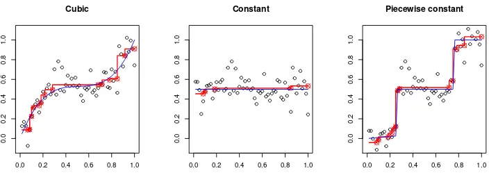
The above characterization of the isotonic LSE shows that ˆθ is piecewise constant, and in each “block” (i.e., region of constancy) it is the average of the response values (within the block); see [106, Chapter 1]. However, the blocks, their lengths and their positions, are chosen adaptively by the algorithm, the least squares procedure. If θi∗ = f(xi) for some design points 0 ≤ x1 < · · · < xn ≤ 1, then we can define the isotonic LSE of f as the piecewise constant function ˆfn: [0,1]→R which has jumps only at the design points and such that ˆfn(xi) = ˆθi for each i = 1, . . . , n. Figure 1 shows three different scatter plots, for three different regression functionsf, with the fitted isotonic LSEs ˆfn. Observe that for the leftmost plot the block-sizes (of the isotonic LSE) vary considerably with the change in slope of the underlying function f — the isotonic LSE, ˆfn, is nearly constant in the interval [0.3,0.7] where f is relatively flat whereas ˆfn has many small blocks towards the boundary of the covariate domain where f has large slope. This highlights the adaptive nature of the isotonic LSE ˆfn and also provides some intuition as to why the isotonic LSE adapts to piecewise constant nondecreasing functions with not too many constant pieces. Moreover, in some sense, ˆfn can be thought of as a kernel estimator (with the box kernel) or a ‘regressogram’ ([120]), but with a varying bandwidth/window.
2.1. Worst case risk bound
The worst case risk bound for the isotonic LSE is given by the following inequality. Under the assumption that the errorsε1, . . . , εnare i.i.d. with mean zero and varianceσ2, the risk of the isotonic LSE satisfies the bound (see [129]):
R(ˆθ, θ∗)≤C
σ2V(θ∗) n
2/3
+Cσ
2log(en)
n (12)
0.0 0.2 0.4 0.6 0.8 1.0
0.0
0.2
0.4
0.6
0.8
1.0
Cubic
0.0 0.2 0.4 0.6 0.8 1.0
0.0
0.2
0.4
0.6
0.8
1.0
Constant
0.0 0.2 0.4 0.6 0.8 1.0
0.0
0.2
0.4
0.6
0.8
1.0
Piecewise constant
Fig 1: Plots of Y (circles), ˆθ (red), and θ∗ (blue) for three different f’s: (i) cubic polynomial
(left plot), (ii) constant (middle plot), and (iii) piecewise constant. Here n = 60, and ε∼Nn(0, σ2In) withσ= 0.1. HereIn denotes the identity matrix of ordern.
multiplicative factor. This shows that the rate of estimating any monotone function (under theℓ2-loss) isn−2/3. Moreover, (12) gives the explicit dependence of the risk on the variation
of θ∗ (and on σ2).
The second term on the right side of (12) is also interesting — when V(θ∗) = 0, i.e.,θ∗ is a constant sequence, (12) shows that the risk of the isotonic LSE scales like logn/n. This is a consequence of the fact that ˆθ chooses its blocks (of constancy) adaptively depending on the data. When θ∗ is the constant sequence, ˆθ has fewer blocks (in fact, it has of the order of lognblocks; see e.g., [92, Theorem 1]) and some of the blocks will be very large (see e.g., the middle plot of Figure 1), so that averaging the responses within the large blocks would yield a value very close to the grand mean ¯Y = (Pn
i=1yi)/n (which has risk σ2/n in this problem). Thus (12) already illustrates the adaptive nature of the LSE — the risk of the LSE ˆθ changes depending on the “structure” of the true θ∗. In the next subsection (see (13)) we further highlight this adaptivenature of the LSE.
Remark 2.1. To the best of our knowledge, inequality (12)first appeared in [92, Theorem 1] who proved it under the assumption that the errorsε1, . . . , εnare i.i.d.N(0, σ2). Zhang [129]
proved (12) for much more general errors including the case when ε1, . . . , εn are i.i.d. with mean zero and variance σ2. The proof we give (in Section 7.2) follows the arguments of
[129]. Another proof of an inequality similar to (12) for the case of normal errors has been given recently by [23] who proved it as an illustration of a general technique for bounding the risk of LSEs.
Remark 2.2. The LSE over bounded monotone functions also satisfies the bound (12)and has been observed by many authors including [99, 121, 36]. Proving this result is easier, however, because of the presence of the uniform bound on the function class (such a bound is not present for the isotonic LSE). It must also be kept in mind that the bounded isotonic LSE comes with a tuning parameter that needs to chosen by the user.
Remark 2.3. Inequality (12)also implies that the isotonic LSE achieves the risk(σ2V /n)2/3
for θ∗ ∈ IV :={θ∈ I :θn−θ1≤V}(as long as V is not too small) without any knowledge
in the rangeσ/√n.V .σn(see e.g., [25, Theorem 5.3]). Therefore, in this wide range of V, the isotonic LSE is minimax (up to constant multiplicative factors) over the class IV. This is especially interesting because the isotonic LSE does not require any knowledge of V. This illustrates another kind of adaptation of the isotonic LSE; further details on this can be found in [28].
2.2. Adaptive risk bounds
As the isotonic LSE fit is piecewise constant, it may be reasonable to expect that when θ∗ is itself a piecewise constant (with not too many pieces), the risk of ˆθ would be small. The rightmost plot of Figure 1 corroborates this intuition. This leads us to our second type of risk bound for the LSE. For θ∈ I, letk(θ)≥1 denote the number of constant blocks of θ, i.e., k(θ) is the integer such that k(θ)−1 is the number of inequalities θi ≤θi+1 that are
strict, for i= 1, . . . , n−1 (the number of jumps ofθ).
Theorem 2.1. Under the assumption thatε1, . . . , εnare i.i.d. with mean zero and variance σ2 we have
R(ˆθ, θ∗)≤ inf θ∈I
1 nkθ
∗−θk2+4σ2k(θ)
n log en k(θ)
(13)
for every θ∗ ∈Rn.
Note that θ∗ in Theorem 2.1 can be any arbitrary vector inRn (it is not required that θ∗ ∈ I). An important special case of inequality (13) arises when θ is taken to be θ∗ in order to obtain:
R(ˆθ, θ∗)≤ 4σ
2k(θ∗)
n log en
k(θ∗). (14)
It makes sense to compare (14) with the worst case risk bound (12). Suppose, for ex-ample, θj∗ = 1{j > n/2} (here 1 denotes the indicator function) so that k(θ∗) = 2 and V(θ∗) = 1. Then the risk bound in (12) is essentially (σ2/n)2/3 while the right side of (14)
is (8σ2/n) log(en/2) which is much smaller than (σ2/n)2/3. More generally, ifθ∗is piecewise constant with kblocks then k(θ∗) =kso that inequality (14) implies that the risk is given by the parametric ratekσ2/nwith a logarithmic multiplicative factor of 4 log(en/k) — this
is a much stronger bound compared to (12) whenk is small.
Inequality (14) is an example of an oracle inequality. This is because of the following. Let ˆθOR denote the oracle piecewise constant estimator of θ∗ which estimates θ∗ by the mean of Y in each constant block of θ∗ (note that ˆθOR uses knowledge of the locations of the constant blocks of θ∗ and hence is an oracle estimator). It is easy to see then that the risk of ˆθOR is given by
R(ˆθOR, θ∗) = σ
2k(θ∗)
n . As a result, inequality (14) can be rewritten as
R(ˆθ, θ∗)≤
4 log en k(θ∗)
R(ˆθOR, θ∗). (15)
the isotonic LSE, which uses no knowledge of k(θ∗) and the positions of the blocks, has essentially the same risk performance as the oracle piecewise-constant estimator (up to the multiplicative logarithmic factor 4 log(en/k(θ∗))). This is indeed remarkable!
Inequality (13) can actually be viewed as a more general oracle inequality where the behavior of the isotonic LSE is compared with oracle piecewise constant estimators even when θ∗ ∈ I/ . We would like to mention here that, in this context, (13) is referred to as a sharp oracle inequality because the leading constant in front of thekθ∗−θk2/nterm on the
right-hand side of (13) is equal to one. We refer to [16] for a detailed explanation of oracle and sharp oracle inequalities.
Based on the discussion above, it should be clear to the reader that the adaptive risk bound (13) complements the worst case bound (12) as it gives much finer information about how well any particular θ∗ (depending on its ‘complexity’) can be estimated by the LSE ˆθ.
Remark 2.4 (Model misspecification). As already mentioned, the sharp oracle inequal-ity (13) needs no assumption on θ∗ (which can be any arbitrary vector in Rn), i.e., the inequality holds true even when θ∗ ∈ I/ . See [25, Section 6] for another way of handling model misspecification, where θˆis compared with the “closest” element to θ∗ in I (and not θ∗).
Remark 2.5. To the best of our knowledge, an inequality of the form (13) first explicitly appeared in [25, Theorem 3.1] where it was proved that
R(ˆθ, θ∗)≤4 inf θ∈I
1 nkθ
∗−θk2+4σ2k(θ)
n log en k(θ)
(16)
under the additional assumption that θ∗ ∈ I. The proof of this inequality given in [25] is based on ideas developed in [129]. Note the additional constant factor of 4 in the above inequality compared to (13).
Under the stronger assumption ε∼Nn(0, σ2In), Bellec [16, Theorem 3.2] improved (16) and proved that
R(ˆθ, θ∗)≤inf θ∈I
1 nkθ
∗−θk2+σ2k(θ)
n log en k(θ)
, (17)
for every θ∗ ∈ Rn. A remarkable feature of this bound is that the multiplicative constants involved are all tight, which implies, in particular, that
R(ˆθ, θ∗)≤inf θ∈I
1 nkθ
∗−θk2+Cσ2k(θ)
n log en k(θ)
cannot hold for everyθ∗ ifC <1. This follows from the fact that whenθ∗ = (0,0, . . . ,0)∈ I and ε∼Nn(0, σ2In), the riskR(ˆθ, θ∗)exactly equals σ2Pnj=11/j ≍σ2logn; see [16] for an
explanation. It must be noted that this implies, in particular, that the logarithmic term in these adaptive risk bounds cannot be removed.
Note that inequality (13) has an additional factor of 4 compared to (17) on the second term in the right-hand side. This is because the errors ε1, . . . , εn can be non-Gaussian in
Theorem 2.1.
an approach will lead to additional logarithmic terms on the right hand side of (12) (see e.g., [25, Theorem 4.1]).
2.2.1. Adaptive Risk Bounds for R(p)(ˆθ, θ∗).
The risk bound (13) (or more specifically (15)) implies that the isotonic LSE pays a log-arithmic price in risk compared to the oracle piecewise constant estimator. This fact is strongly tied to the fact that the risk is measured via squared error loss (as in (9)). The story will be different if one measures risk under ℓp-metrics for p6= 2. To illustrate this, we shall describe adaptive bounds for the risk R(p)(ˆθ, θ∗) defined in (10).
The following result bounds the risk R(p)(ˆθ, θ∗) assuming that θ∗ ∈ I. The risk bounds involve a positive constant Cp that depends on p alone. Explicit expressions for Cp can be gleaned from the proof of Theorem 2.2(in Section 7.4).
Theorem 2.2. Assume that the errors ε1, . . . , εn are i.i.d. N(0, σ2). Fix θ∗ ∈ I and let p ≥ 1, p 6= 2. Let k denote the number of constant blocks of θ∗ and let the lengths of the blocks be denoted by n1, . . . , nk. We then have
R(p)(ˆθ, θ∗)≤Cpσ p
n k
X
i=1
n(2−p)+/2
i ≤Cpσp
k n
min(p,2)/2
(18)
where Cp is a positive constant that depends on p alone.
Remark 2.7. As stated, Theorem 2.2 appears to be new even though its conclusion is implicit in the detailed risk calculations of [129] for isotonic regression. Zhang’s [129] argu-ments also seem to indicate that the bound (18)should be tight up to constant multiplicative terms involving p. We have assumed that ε1, . . . , εn are normal in Theorem 2.2 but it is
possible to allow non-Gaussian errors by imposing suitable moment conditions.
Let us now compare the isotonic LSE to the oracle piecewise constant estimator ˆθOR (introduced in the previous subsection) in terms of the ℓp-risk. It is easy to verify that the risk of ˆθOR under theℓp-loss is given by
R(p)(ˆθOR, θ∗) = (E|η|p)σp1 n
k
X
i=1
n(2i −p)/2 (19)
for every p >0 where η:=ε1/σ is standard normal.
Comparing (18) and (19), we see that the isotonic LSE performs at the same rate (up to constant multiplicative factors) as the oracle piecewise constant estimator for 1≤p <2 (there is not even a logarithmic price for these values of p). When p= 2, as seen from (15), the isotonic LSE pays a logarithmic price of 4 log(en/k(θ∗)). For p > 2 however, there is a significant price that is paid. For example, if all the constant blocks have roughly equal size, then the oracle estimator’s risk, when p >2, equals (k/n)p/2 while the bound in (18) is of order k/n.
restricted additive models (Example 1.5). In each of these problems, we describe results related to the performance of the LSEs. The reader will notice that the risk results are not as detailed as compared to the isotonic regression results of the previous section.
3.1. Convex Regression
Let us consider Example 1.3where the goal is to estimate a convex function f : [0,1]→ R from regression data as in (1). The convex LSE ˆθ is defined as the projection ofY onto the closed convex cone K (see (6)). This estimator was first proposed in [69] for the estimation of production functions and Engel curves. It can be shown that ˆθ is piecewise affine with knots only at the design points; see [58, Lemma 2.6]. The accuracy of the LSE, in terms of the risk R(ˆθ, θ∗) (defined in (9)), was first studied in [64] followed by [25,16,24]. These results are summarized below. Earlier results on the risk under a supremum loss can be found in [66,40].
Suppose that ε ∼ Nn(0, σ2In). In [24], the following worst case risk bound for ˆθ was given (when xi=i/n are the ordered design points):
R(ˆθ, θ∗)≤C σ
2p
T(θ∗) n
!4/5
+C σ
2
n4/5 (20)
where C > 0 is a universal constant and T(θ∗) is a constant depending on θ∗ (like V(θ∗) in (12) for isotonic regression). Roughly speaking,T(θ∗) measures the “distance” ofθ∗ from the set of all affine (functions) sequences. Formally, LetLdenote the subspace ofRnspanned by the constant vector (1, . . . ,1) and the vector (1,2, . . . , n); i.e., L is the linear subspace of affine sequences. Let PL denote the orthogonal projection matrix onto the subspace L and let β∗ := (In−PL)θ∗. Then T(θ∗) := max1≤i≤nβi∗−min1≤i≤nβi∗. Observe that when θ∗ itself is an affine sequence (which is also a convex sequence), thenT(θ∗) = 0.
The risk bound (20) shows that the risk of the convex LSE is bounded above byn−4/5. Inequality (20) improved a result in [64], which had a similar bound but with an additional multiplicative logarithmic factor (inn). Comparing with (12), it is natural to conjecture that the second term in (20) can be improved to Cσ2(log(en))/n but this has not been proved so far. Another feature of (20) is that the errors are assumed to be Gaussian; it might be possible to extend them to sub-Gaussian errors but this is still a strong assumption compared to the corresponding result for isotonic regression (see (12)) which holds without distributional assumptions.
The proof of (20) (and other worst case risk bounds like (20) for shape-restricted re-gression problems under Gaussian/sub-Gaussian errors) involves tools from the theory of Gaussian processes like chaining and Dudley’s entropy bound and crucially relies on an ac-curate ‘size’ measure of the underlying class (e.g., ‘local’ balls ofK) as captured by its metric entropy; see Section 3.5 for a broad outline of the proof strategy. Although the main idea of the proof is simple, deriving appropriate bounds on the metric entropy of the underlying class can be challenging.
q(θ)≥1 denote the number of affine pieces ofθ; i.e.,q(θ) is an integer such that q(θ)−1 is the number of inequalities in (6) that are strict. This adaptive behavior can be illustrated through the following risk bound:
R(ˆθ, θ∗)≤ inf θ∈K
1 nkθ
∗
−θk2+8σ
2q(θ)
n log en q(θ)
. (21)
This inequality has been proved by [16, Section 4] improving earlier results of [64,25] which had superfluous multiplicative constants. Note that this bound holds forε∼N(0, σ2In). It is not known if the bounds holds for non-Gaussian errors (compare this with the corresponding inequality (13) for isotonic regression which holds without distributional assumptions on the errors). Let us also note that risk bounds for the LSE under theR(p)(ˆθ, θ∗) risk (defined in (10)) are not available for convex regression.
3.2. Isotonic regression on a partially ordered set
We now turn our attention to Example1.2where the covariates are partially ordered and the goal is to estimate the order preserving (isotonic) regression function. The book Robertson et al. [106, Chapter 1] gives a nice overview of the characterization and computation of LSEs in such problems along with their applications in statistics. However, not much is known in terms of rates of convergence for these LSEs beyond the example of coordinate-wise nondecreasing ordering introduced in Example 1.2.
In this subsection we briefly review the main results in [26] which considers estimation of a bivariate (d= 2) coordinate-wise nondecreasing regression function. An interesting recent paper [65] has extended these results to all dimensionsd≥2 (see Remark 3.1). Estimation of bivariate coordinate-wise nondecreasing functions has applications and connections to the problem of estimating matrices of pairwise comparison probabilities arising from pairwise comparison data ([29,113]) and to seriation ([43]).
As the distribution of the design points xi complicate the analysis of shape-restricted LSEs, especially when d > 1, for simplicity, we consider the regular uniform grid design. This reduces the problem to estimating an isotonic ‘matrix’ θ∗ := (θij∗) ∈ Rn1×n2 from
observations
yij =θij∗ +εij, fori= 1, . . . , n1, j= 1, . . . , n2,
where θ∗ is constrained to lie in
M:={θ∈Rn1×n2 :θij ≤θ
kl wheneveri≤kand j≤l},
and the random errors εij’s are i.i.d. N(0, σ2), with σ2 > 0 unknown. We refer to any matrix inMas an isotonic matrix. LettingY := (yij) denote the matrix (of ordern1×n2;
n:=n1n2) of the observed responses, the LSE ˆθis defined as the minimizer of the squared
Frobenius norm, kY −θk2, overθ∈ M, i.e.,
ˆ
θ:= arg min θ∈M
n1 X
i=1
n2 X
j=1
(yij−θij)2. (22)
The goal now is to formulate both the worst case and adaptive risk bounds for the matrix isotonic LSE ˆθ in estimatingθ∗. In [26, Theorem 2.1] it was shown that
R(ˆθ, θ∗)≤C
r
σ2D(θ∗) n (logn)
4+σ2
n(logn)
8
!
(23)
for a universal constantC >0, whereD(θ∗) := (θn∗1n2−θ11∗ )2. The above bound shows that
when the ‘variation’ D(θ∗) of θ∗ is non-zero, the risk of ˆθ decays at the rate n−1/2, while
when D(θ∗) = 0 (i.e., θ∗ is a constant), the risk is (almost) parametric. The above bound probably has superfluous logarithmic factors (see [65]).
To describe the adaptive risk bound for the matrix isotonic LSE we need to introduce some notation. A subset A of {1, . . . , n1} × {1, . . . , n2} is called a rectangleif A={(i, j) : k1 ≤i≤l1, k2 ≤ j ≤l2} for some 1 ≤k1 ≤ l1 ≤n1 and 1≤ k2 ≤l2 ≤ n2. A rectangular
partition of {1, . . . , n1} × {1, . . . , n2} is a collection of rectangles π= (A1, . . . , Ak) that are disjoint and whose union is {1, . . . , n1} × {1, . . . , n2}. The cardinality of such a partition,
|π|, is the number of rectangles in the partition. The collection of all rectangular partitions of {1, . . . , n1} × {1, . . . , n2} will be denoted byP. For θ ∈ M and π = (A1, . . . , Ak) ∈ P, we say that θ is constant onπ if {θij : (i, j)∈Al} is a singleton for eachl = 1, . . . , k. We definek(θ), forθ∈ M, as the “number of rectangular blocks” ofθ, i.e., the smallest integer k for which there exists a partitionπ∈ P with|π|=k such thatθ is constant onπ. In [26, Theorem 2.4] the following adaptive risk bound was stated:
R(ˆθ, θ∗)≤ inf θ∈M
kθ∗−θk2
n +
Cσ2k(θ) n (logn)
8
. (24)
where C >0 is a universal constant.
In [26] the authors also established a property of the LSE that they termed ‘variable’ adaptation. Let In1 :={θ∈R
n1 :θ
1 ≤ · · · ≤θn1}. Suppose θ
∗= (θ∗
ij)∈ I has the property that θij∗ only depends on i, i.e., there exists θ∗∗ ∈ In1 such that θ
∗
ij = θi∗∗ for every i and j. If we knew this fact about θ∗, then the most natural way of estimating it would be to perform vector isotonic estimation based on the row-averages ¯y := (¯y1, . . . ,y¯n1), where
¯
yi :=Pnj=12 yij/n2, resulting in an estimator ˘θofθ∗∗. Note that the construction of ˘θrequires
the knowledge that all rows ofθ∗ are constant. As a consequence of the adaptive risk bound (24), it was shown in [26, Theorem 2.4] that the matrix isotonic LSE ˆθ achieves the same risk bounds as ˘θ, up to additional logarithmic factors. This is remarkable because ˆθuses no special knowledge onθ∗; it automatically adapts to intrinsic dimension ofθ∗.
Remark 3.1 (Extension to d ≥ 2). The recent paper Han et al. [65] has studied d -dimensional isotonic regression for general d≥ 1 and proved versions of inequalities (23) and (24). Their results imply, in particular, that the worst case risk behavior as well as adaptive risk behavior of the isotonic LSE changes significantly for d≥ 3 compared to the behavior for d ≤ 2. They also obtained results for the isotonic LSE under random design settings.
3.3. Unimodal Regression
In this subsection we summarize the two kinds of risk bounds known for the LSE in unimodal (decreasing and then increasing) regression, introduced in Example1.4. The unimodal LSE ˆθ is defined as any projection ofY ontoU, a finite union of the closed convex cones described in Example1.4. It is known that ˆθis piecewise constant with possible jumps only at the design points. Once the mode of the fitted LSE is known (and fixed), ˆθ is just the nonincreasing (isotonic) LSE fitted to the points to the left of the mode and nondecreasing (isotonic) LSE fitted to the points on the right of the mode.
As in isotonic regression, the unimodal LSE ˆθ exhibits adaptive behavior. In fact, the risk bounds for the unimodal LSE ˆθare quite similar to those obtained for the isotonic LSE. The two kinds of risk bounds are given below (under the assumption that ε∼Nn(0, σ2In)):
R(ˆθ, θ∗)≤C
σ2S(θ∗) n
2/3
+C σ
2
n2/3, whereθ
∗∈ U, (25)
and
R(ˆθ, θ∗)≤C inf θ∈U
1 nkθ
∗
−θk2+Cσ
2(k(θ) + 1)
n log
en k(θ) + 1
(26)
where k(θ) is the number of constant blocks of θ, S(θ∗) := maxi,j|θi∗−θj∗|is the range of θ∗ and C >0 is a universal constant.
The worst case risk bound (25) is given in [27, Theorem 2.1] while the adaptive risk bound (26) is a consequence of [16, Theorem A.4] (after integrating the tail probability). The proof of (25) (given in [27, Theorem 2.1]) is based on the general theory of least squares outlined in Section 3.5; also see [23, Theorem 2.2]. It shows that a unimodal regression function can also be estimated at the same rate as a monotone function. The adaptive risk bound (26), although being similar in spirit to that of the isotonic LSE, is weaker than (17) (obtained for the isotonic LSE). Note that inequality (26) is not sharp (i.e., the leading constant on the right side of (26) is not 1); in fact it is not known whether a sharp oracle inequality can be constructed forR(ˆθ, θ∗) (see [16]). The proof of the adaptive risk bound is also slightly more involved than that of Theorem2.1; the fact that the underlying parameter space U is non-convex complicates the analysis.
3.4. Shape-restricted additive models
Given observations (x1, y1), . . . ,(xn, yn) where{xi= (xij,1≤j≤d)}ni=1 ared-dimensional
design points and y1, . . . , yn are real-valued, the additive model (see e.g., [68,86]) assumes
that
yi =µ∗+ d
X
j=1
fj∗(xij) +εi fori= 1, . . . , n
where µ∗ ∈ R is an unknown intercept term, f∗
1, . . . , fd∗ are unknown univariate functions satisfying
1 n
n
X
i=1
and ε1, . . . , εn are unobserved mean-zero errors. Assumption (27) is necessary to ensure the identifiability of f1∗, . . . , fd∗. We focus our attention to shape-restricted additive models where it is assumed that eachfj∗ obeys a known qualitative restriction such as monotonicity or convexity which is captured by the assumption thatfj∗ ∈ Fjfor a known class of functions
Fj. One of the main goals in additive modeling is to recover each individual functionfj∗ ∈ Fj forj = 1, . . . , d.
The LSEs ˆµ,fjˆ ofµ∗, fj∗, forj = 1, . . . , dare defined as minimizers of the sum of squares criterion, i.e.,
(ˆµ,fˆ1, . . . ,fˆd) := arg min n
X
i=1
yi−µ− d
X
j=1
fj(xij)
2
(28)
under the constraints µ ∈ R, fj ∈ Fj,Pn
i=1fj(xij) = 0 forj = 1, . . . , d. It is natural to compare the performance of these LSEs to the corresponding oracle estimators defined in the following way. For each k= 1, . . . , d, the oracle estimator ˆfkOR is defined as
ˆ
fkOR:= arg min fk
n
X
i=1
yi−µ∗−
X
j6=k
fj∗(xij)−fk(xik)
2
, (29)
where fk ∈ Fk and satisfies Pni=1fk(xik) = 0. In other words, ˆfkOR assumes knowledge of fj∗, forj 6=k, and µ∗, and performs least squares minimization only overfk∈ Fk.
A very important aspect about shape-restricted additive models is that it is possible for the LSE ˆfk to be close to the oracle estimator ˆfkOR, for each k = 1, . . . , d. Indeed, this property was proved by Mammen and Yu [89] under certain assumptions for additive isotonic regression where each function fj is assumed to be monotone. Specifically, [89] worked with a random design setting where the design points are assumed to be i.i.d. from a Lipschitz density that is bounded away from zero and infinity on [0,1]d(this is a very general setting which allows for non-product measures). They also assumed that each function fj is differentiable and strictly increasing. Although the design restrictions in this result are surprisingly minimal, we believe that the assumptions on the fj’s can be relaxed. In particular, this result should hold when fj’s are piecewise constant and even under more general shape restrictions such as convexity.
Our intuition is based on the following (trivial) observation that there exist design con-figurations where the LSE ˆfkis remarkably close to ˆfkOR for eachk= 1, . . . , dunder almost no additional assumptions. The simplest such instance is when the design points take values in a uniform grid. In this case, it is easy to see that ˆfk is exactly equal to ˆfkOR as shown below. For simplicity, assume that d= 2 and that the design points are coming from a grid in [0,1]2. It is convenient then to index the observations by (i
1, i2) wherei1= 1, . . . , n1 and
i2 = 1, . . . , n2 (n=n1×n2). The design points will be given by xi1,i2 = (i1/n1, i2/n2) and
the observation model can be written as
yi1,i2 =µ
∗+f∗
1(i1/n1) +f2∗(i2/n2) +εi1,i2, (30)
fori1 = 1, . . . , n1, i2 = 1, . . . , n2.The following result is proved in Section7.5.
Lemma 3.1. Consider model (30) where fk∗ ∈ Fk, for k = 1,2. Suppose that fˆ1 and fˆ2
denote the LSEs off1∗ andf2∗ respectively, as defined in (28). Also, let the oracle estimators be as defined fˆOR
Note that we have made no assumptions at all onF1andF2. Thus under the regular grid design in [0,1]d, the LSEs off1 andf2 are exactly equal to the oracle estimates. For general
design configurations, it might be much harder to relate the LSEs to the corresponding oracle estimators. Nevertheless, the aforementioned phenomenon for gridded designs allows us to conjecture that the closeness of ˆfk to ˆfkOR must hold in much greater generality than has been observed previously in the literature.
It may be noted that the risk behavior of ˆfkORis easy to characterize. For example, when fk∗ is assumed to be monotone, ˆfkOR will satisfy risk bounds similar to those described in Section 2. Likewise, when fk∗ is assumed to be convex, then ˆfkOR will satisfy risk bounds described in Subsection 3.1. Thus, when ˆfk is close to ˆfkOR (which we expect to happen under a broad set of design configurations), it is natural to expect that ˆfk will satisfy such risk bounds as well.
3.5. General theory of LSEs
In this section, we collect some general results on the behavior of the LSEs that are useful for proving the risk bounds described in the previous two sections. These results apply to LSEs that are defined by (7) for a closed convex constraint setC. Convexity ofCis crucial here (in particular, these results do not directly apply to unimodal regression where the constraint set is non-convex; see Section 3.3). We assume that the observation vector Y =θ∗+ε for a mean-zero random vectorε. Except in Lemma 3.4, we assume thatε∼Nn(0, σ2In).
The first result reduces the problem of bounding R(ˆθ, θ∗) to controlling the expected supremum of an appropriate Gaussian process. This result was proved by Chatterjee [23] (see [30,122] for extensions to penalized LSEs).
Lemma 3.2 (Chatterjee). Consider the LSE (7) for a fixed closed convex set C. Assume that Y =θ∗+εwhere ε∼Nn(0, σ2In) and θ∗ ∈ C. Let us define the functiongθ∗ :R+ →R as
gθ∗(t) :=E
"
sup θ∈C:kθ−θ∗k≤th
ε, θ−θ∗i
#
− t 2
2. (31)
Let tθ∗ be the point in [0,∞) where t7→gθ∗(t) attains its maximum (existence and unique-ness of tθ∗ are proved in [23, Theorem 1.1]). Then there exists a universal positive constant C such that
R(ˆθ, θ∗)≤ C
n max t
2
θ∗, σ2
. (32)
Remark 3.2. Chatterjee [23] actually proved that kθˆ−θ∗k is tightly concentrated around tθ∗. The bound (32) is an easy consequence of this concentration result.
Lemma 3.2 reduces the problem of bounding R(ˆθ, θ∗) to that of bounding tθ∗. For this latter problem, [23, Proposition 1.3] observed that
tθ∗ ≤t∗∗ whenever t∗∗>0 andgθ∗(t∗∗)≤0.
entropy bound (see e.g., [119, Chapter 2]) which is given below. This bound involves covering numbers. For a subset K ⊆Rn and ǫ >0, let N(ǫ, K) denote the ǫ-covering number of K under the Euclidean metric k · k (i.e., N(ǫ, K) is the minimum number of closed balls of radius ǫ required to coverK). The logarithm of N(ǫ, K) is known as the ǫ-metric entropy of K. Also, for eachθ∗∈ C and t >0, let
B(θ∗, t) :={θ∈ C :kθ−θ∗k ≤t}
denote the ball of radius t aroundθ∗. Observe that the supremum in the definition in (31) is over all θ∈B(θ∗, t). Dudley’s entropy bound leads to the following upper bound for the expected Gaussian supremum appearing in the definition of gθ∗(t).
Lemma 3.3 (Chaining). For every θ∗ ∈ C and t >0, E
"
sup θ∈B(θ∗,t)h
ε, θ−θ∗i
#
≤σ inf
0<δ≤2t
12
Z 2t
δ
p
logN(ǫ, B(θ∗, t))dǫ+ 4δ√n
.
Remark 3.3. Dudley’s entropy bound is not always sharp. More sophisticated generic chaining arguments exist which gives tight bounds (up to universal multiplicative constants) for suprema of Gaussian processes; see [119].
Lemma3.2and Lemma3.3present one way of boundingR(ˆθ, θ∗). This involves control-ling the metric entropy of subsets of the constraint setC of the formB(θ∗, t). This method is useful but works only for the case of Gaussian/sub-Gaussian errors.
Let us now present another result which is useful for proving adaptive risk bounds under misspecification. We shall now work with general error distributions for ε that are not necessarily Gaussian (we only assume that E(ε) = 0). This result essentially states for boundingR(ˆθ, θ∗), it is possible to work withtangent cones associated withC instead ofC. It is easier to deal with cones as opposed to general closed convex sets which leads to the usefulness of this result.
For a closed convex setC and θ∈ C, thetangent cone of C atθis defined as
TC(θ) := Closure{t(η−θ) :t≥0, η ∈ C}.
Informally, TC(θ) represents all directions in which one can move fromθ and still remain in
C. The following lemma relates the riskR(ˆθ, θ∗) to tangent cones.
Lemma 3.4. LetC be a closed convex set inRn. Let θ∗ ∈Rnand suppose that Y =θ∗+σZ for some mean-zero random vector Z with EkZk2<∞. Then,
E
kθˆ−θ∗k2
≤inf θ∈C
n
kθ∗−θk2+σ2E
kΠTC(θ)(Z)k2
o
, (33)
where ΠTC(θ)(Z) denotes the projection of Z onto the closed convex coneTC(θ).
Some remarks on this lemma are given below.
Remark 3.4 (Statistical dimension). When Z ∼Nn(0, In) and K is a closed convex cone in Rn, the quantity
δ(K) :=E
kΠK(Z)k2
=E
hZ,ΠK(Z)i
=E
"
sup θ∈K:kθk≤1h
Z, θi2
#
has been termed the statistical dimension ofK by Amelunxen et al. [2]. Therefore, whenZ ∼
Nn(0, In),inequality (33) bounds the risk R(ˆθ, θ∗) of the LSE via the statistical dimension of the tangent cones TC(θ).
Remark 3.5 (No distributional assumptions). There are no distributional assumptions on Z for (33) to hold. In particular, the components of Z can be arbitrarily dependent and non-Gaussian (as long as EkZk2 <∞). This result first appeared in [16, Proposition 2.1] who stated it assuming that Z ∼Nn(0, In) but an examination of the proof reveals that the Gaussian assumption is not necessary.
Remark 3.6. When θ∗ ∈ C, then one can take θ=θ∗ in the right side of (33) to deduce that
Ekθˆ−θ∗
k2≤σ2EkΠTC(θ∗)(Z)k2. (34) This inequality (34)was first proved by [101]. Bellec [16] extended it to the case when θ∗∈ C/ by proving Lemma 3.4.
Remark 3.7 (Tightness). A remarkable fact proved by Oymak and Hassibi [101] is that lim
σ↓0
1
σ2Ekθˆ−θ
∗k2=EkΠ
TC(θ∗)(Z)k2 when θ∗ ∈ C. (35)
Analogues of this inequality when θ∗ ∈ C/ have been recently proved in [42]. The equality in (35) implies that if rn(θ), for θ ∈ C, is any rate term controlling the adaptive behavior of the LSE in the following sense:
Ekθˆ−θ∗
k2≤ inf θ∈C
kθ∗−θk2+σ2rn(θ) for everyθ∗ ∈Rn
then it necessarily must happen that
rn(θ)≥EkΠTC(θ)(Z)k2 for everyθ∈ C.
Thus one loses nothing when working with tangent cones (i.e., focussing on boundingEkΠTC(θ)(Z)k2)
to prove adaptive risk bounds.
We shall show how to apply Lemma3.4to prove the adaptive risk bound (13) in Section 7.1. Lemma3.4is also crucially used in [16] to prove the adaptive risk bound (21) for convex regression. Lemma3.4also has applications beyond shape-restricted regression. It has been recently used to prove risk bounds for total variation denoising and trend filtering (see [63]).
4. Inference with shape-restricted functions
Till now we have focused our attention on (global) risk properties of shape-restricted LSEs. In this section we investigate the pointwise limiting behavior of the estimators. By the pointwise behavior we mean the distribution of the LSE ˆfnat a fixed point (sayt), properly normalized. Developing asymptotic distribution theory for the LSEs turns out to be rather non-trivial, mainly because there is no closed form simple expression for the LSEs; all the properties of the estimator have to be teased out from the general characterization (8).
parameters (that are difficult to estimate). As before, analyzing the isotonic LSE is probably the simplest, and we will work with this example in Section 4.1. In Section4.2 we develop bootstrap and likelihood based methods for constructing (asymptotically) valid pointwise confidence intervals, for the isotonic regression functionf, that bypass estimation of nuisance parameters. Section 4.3 deals with the case when f is convex — we sketch a proof of the pointwise limiting distribution of the convex LSE. Not much is known in this area beyond d= 1 for any of the shape-restricted LSEs discussed in the Introduction.
4.1. Pointwise limit theory of the LSE in isotonic regression
Let us recall the setup in (1) wheref is now an unknown nondecreasing function. Further, for simplicity, letxi=i/n, fori= 1, . . . , n, be the ordered design points and we assume that ε1, . . . , εnare i.i.d. mean zero errors with finite varianceσ2 >0. The above assumptions can
be relaxed substantially, e.g., we can allow for dependent, heteroscedastic errors and the xi’s can be any sequence whose empirical distribution converges to a probability measure on [0,1]; see e.g., [3], [123, Section 3.2.15].
We start with another useful characterization of the isotonic LSE ([15, Theorem 1.1]). Define the cumulative sum diagram (CSD) as the continuous piecewise affine functionFn: [0,1]→R(with possible knots only ati/n, fori= 1, . . . , n) for which
Fn(0) := 0, and Fn
i
n
:= 1 n
i
X
j=1
yj, fori= 1, . . . , n. (36)
For any function g:I →R, whereI ⊂Ris an interval, we denote by ˜g thegreatest convex minorant (GCM) of g (on I), i.e., ˜g is the largest convex function sitting below g. Thus,
˜
Fn denotes the GCM of Fn (on the interval [0,1]). Let ˆfn : (0,1] → R be defined as the left-hand derivative of the GCM of the CSD; i.e.,
ˆ
fn:= [ ˜Fn]′ ≡F˜n′,
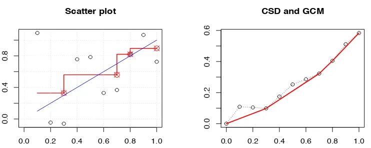
the left-hand slope of ˜Fn. Then, it can be shown that (see e.g., [106, Chapter 1]) the isotonic LSE ˆθis given by ˆθi = ˆfn(i/n), for i= 1, . . . , n. Figure 2 illustrates these concepts from a simple simulation.
Fix 0< t <1 and suppose thatf has a positive continuous derivative f′ on some neigh-borhood of t. The goal is to find the asymptotic distribution of ˆfn(t), properly normalized. We will show that
∆n:=n1/3{fˆn(t)−f(t)}→d κC (37) where C:= arg minh∈R{W(h) +h2} has Chernoff’s distribution (here W(·) is a two-sided
Brownian motion starting from 0) and κ := [4σ2f′(t)]1/3; see e.g., [21, 126, 50, 51]. The first result of this type was derived in [104] for the Grenander estimator — the maximum likelihood estimator of a nonincreasing density in [0,∞) (see [49]). Note that the Chernoff’s random variable Cis pivotal and its quantiles are known; see e.g., [33,62].
4.1.1. Outline of a proof of (37).
0.0 0.2 0.4 0.6 0.8 1.0
0.0
0.4
0.8
Scatter plot
0.0 0.2 0.4 0.6 0.8 1.0
0.0
0.2
0.4
0.6
CSD and GCM
Fig 2: The left panel shows the scatter plot with the fitted function ˆfn (in red) and the true f
(in blue) while the right panel shows the CSD (dashed) along with its GCM (in red). Here n= 10,f(x) =xandε∼Nn(0, σ2In) withσ= 0.5.
section; see [123, Section 3.2.15] for an alternative proof technique that uses the switching relationship, due to Groeneboom [51]. Let us further assume that the i.i.d. errors εi’s have a finite moment generating function near 0. This assumption lets us avoid the use of heavy empirical process machinery and, we hope, will make the main technical arguments simple and accessible to a broader audience.
We consider the stochastic process
Zn(h) :=n2/3[Fn(t+n−1/3h)−Fn(t)−n−1/3hf(t)],
for h ∈[−tn1/3,(1−t)n1/3]. We regard stochastic processes as random elements in D(R),
the space of right continuous functions on Rwith left limits, equipped with the projection σ-field and the topology of uniform convergence on compacta; see [102, Chapters IV and V] for background.
Noting that if uis a bounded function and v is affine then u]+v= ˜u+v, we have
˜
Zn(h) :=n2/3[ ˜F
n(t+n−1/3h)−Fn(t)−n−1/3hf(t)],
forh ∈[−tn1/3,(1−t)n1/3]. By taking the left-derivative of the above process ath= 0 we get (w.p. 1),
∆n= [˜Zn]′(0). (38)
The above relation is crucial, as it relates ∆n, the quantity of interest, to a functional of the process Zn. We study the process Zn (and show its convergence) and apply a (version of) ‘continuous’ mapping theorem (see e.g., [74, pp. 217-218]) to derive the limiting distribution of ∆n.
Let ˇFn: [0,1]→Rbe the continuous piecewise affine function (with possible knots only ati/n, fori= 1, . . . , n) with
ˇ Fn
i
n
:= 1 n
i
X
j=1
fj n
and let F : [0,1]→R be defined as
F(x) :=
Z x
0
f(s)ds.
To study the stochastic process Zn we decompose Zn into the sum of the following three terms:
Zn,1(h) := n2/3[F
n(t+n−1/3h)−Fˇn(t+n−1/3h)−Fn(t) + ˇFn(t)], Zn,2(h) := n2/3[ ˇFn(t+n−1/3h)−F(t+n−1/3h)−Fn(t) +ˇ F(t)],
Zn,3(h) := n2/3[F(t+n−1/3h)−F(t)−n−1/3hf(t)],
Observe thatFn−Fˇnis just the partial sum process, properly normalized. By the Hungarian embedding theorem (see e.g., [75]) we know that the partial sum process is approximated by a Brownian motion process such that
Fn(x)−Fˇn(x) =n−1/2σBn(x) +Rn(x), (39)
where Bn is a Brownian motion on [0,1] and
sup x |
Rn(x)|=O
logn
n
w.p. 1.
Thus,
Zn,1(·) =σWn(·) +op(1),
where the process Wn is defined as Wn(h) := n1/6{Bn(t+n−1/3h)−Bn(t)}, h ∈ R, and Wn ∼ W with W being distributed as a two-sided Brownian motion (starting at 0). This shows that the process Zn,1 converges in distribution toW.
To study Zn,2, observe that as f(·) is continuously differentiable in a neighborhood N
around t, we have (by a simple interpolation bound)
sup x∈N|
ˇ
Fn(x)−F(x)|=O(n−1).
Thus,Zn,2 converges to the zero function. By a simple application of Taylor’s theorem, we
can show thatZn,3 converges, uniformly on compacta, to the function D(h) :=h2f′(t)/2. Combining the above results, we obtain thatZn converges in distribution to the process Z(h) :=σW(h) +h2f′(t)/2, i.e.,
Zn→d Z
in the topology of uniform convergence on compacta. Thus, it is reasonable to expect that
∆n= [˜Zn]′(0)→d [˜Z]′(0).
However, a rigorous proof of the convergence in distribution of ∆n involves a little more than an application of a continuous mapping theorem. The convergence of Zn toZis only under the metric of uniform convergence on compacta. However, the GCM near the origin might be determined by values of the process far away from the origin; the convergence Zn toZ itself does not imply the convergence of [˜Zn]′(0) to [˜Z]′(0). We need to show that ∆n is determined by values of Zn(h) for h in an Op(1) neighborhood of 0; see e.g., [74, pp. 217-218] for such a result with a detailed proof.
4.1.2. Other asymptotic regimes.
Observe that the assumptionf′(t)6= 0 is crucial in deriving the limiting distribution in (37). One may ask, what if f′(t) = 0? Or even simply, what iff is a constant function on [0,1]? In the latter case, we can easily show that, as a stochastic process in [0,1],
√
n{fˆn(t)−f(t)}→d σ[˜B]′(t),
whereBis the standard Brownian motion on [0,1]. The above holds because of the following observations. First note that√n{fn(t)ˆ −f(t)}is the left-hand slope of the GCM of√n(Fn−
F) att(asF is now linear). As√n(Fn−F) converges in distribution to the processσBon D[0,1], we have
√
n{fˆn(t)−f(t)}=√n[F^n−F]′(t)→d σ[˜B]′(t).
The above heuristic can be justified rigorously; see e.g., [55, Section 3.2]. In the related (non-increasing) density estimation problem, [51,22] showed that iff(t) lies on a flat stretch of the underlying function f then the LSE (which is also the nonparametric maximum likeli-hood estimator, usually known as the Grenander estimator) converges to a non-degenerate limit at rate n−1/2, and they characterized the limiting distribution.
If one assumes thatf(j)(t) = 0, forj= 1, . . . , p−1, andf(p)(t)6= 0 (forp≥1), wheref(j)
denotes thej’th derivative off, then one can derive the limiting distribution of ˆfn(t), which now converges at the rate n−p/(2p+1); see e.g., [126, 81]. Note that all the above scenarios illustrate that the rate of convergence of the isotonic LSE ˆfn(t) crucially depends on the the behavior of f around t; this demonstrates the adaptive behavior of the isotonic LSE from a pointwise asymptotics standpoint.
4.2. Constructing asymptotically valid pointwise confidence intervals
Although (37) gives the asymptotic distribution of the isotonic LSE at the pointt, it is not immediately clear how it can be used to construct a confidence interval forf(t) — the lim-iting distribution involves the nuisance parameterf′(t) that needs to be estimated. A naive approach would suggest plugging in an estimator off′(t) in the limiting distribution in (37) to construct an approximate confidence interval. However, as ˆfn is a piecewise constant function, ˆfn′ is either 0 or undefined and cannot be used to estimatef′(t) consistently. This motivates the use of bootstrap and likelihood ratio based methods to construct confidence intervals forf(t). In the following we just assume thatε1, . . . , εni.i.d. mean zero errors with
finite variance.
4.2.1. Bootstrap based inference.
Let us revisit (37) and consider the problem of bootstrapping ˆfnto estimate the distribution of ∆n ∼ Hn (say). Suppose that ˆHn is an approximation of Hn (which will be obtained from bootstrap in this subsection) that can be computed. Then, an approximate 1−α (0< α <1) confidence interval forf(t) would be
where ˆqα denotes the α’th quantile of ˆHn.
In a regression setup there are two main bootstrapping techniques: ‘bootstrapping pairs’ and ‘bootstrapping residuals’. Bootstrapping pairs refers to drawing with replacement sam-ples from the data {(xi, yi) :i= 1, . . . , n}; it is more natural when we have i.i.d. bivariate data from a joint distribution. The residual bootstrap procedure fixes the design pointsxi’s and draws
yi∗:= ˇfn(xi) +ε∗i, i= 1, . . . , n
(the ∗ indicates a data point in the bootstrap sample) where ˇfn is a natural estimator of f in the model, and ε∗i’s are i.i.d. (conditional on the data) having the distribution of the (centered) residuals {yi−fˇn(xi) :i= 1, . . . , n}. Let ˆfn∗ denote the isotonic LSE computed from the bootstrap sample. The bootstrap counterpart of ∆n (cf. (37)) is
∆∗n:=n1/3{fˆn∗(t)−fˇn(t)}.
We now approximate Hn by ˆHn, the conditional distribution of ∆∗n, given the data. Note that a natural candidate for ˇfn in isotonic regression is the LSE ˆfn.
Will this bootstrap approximation (by ˆHn) work? This brings us to the notion of con-sistencyof the bootstrap. Let ddenote the Levy metric or any other metric metrizing weak convergence of distributions. We say that ˆHnisweakly consistentifd(Hn,Hn)ˆ →0 in proba-bility. If the convergence holds with probability 1, then we say that the bootstrap isstrongly consistent. If Hn has a weak limit H, then consistency requires ˆHn to converge weakly to H, in probability; and if H is continuous, consistency requires supx∈R|Hn(x)ˆ −H(x)| →0 in probability.
It is well-known that both the above bootstrap schemes — bootstrapping pairs and bootstrapping residuals with ˇfn= ˆfn— yieldinconsistent estimators ofHn; see [1,110,76, 112,52]. Intuitively, the inconsistency of the residual bootstrap procedure can be attributed to the lack of smoothness of ˆfn. Indeed a version of the residual bootstrap where one considers ˇfn as a smoothed version of ˆfn (that can approximate the nuisance parameter f′(t) consistently) can be shown to be consistent; see e.g., [112]. Specifically, suppose that
ˇ
fn is a sequence of estimators such that
lim n→∞supx∈I
fˇn(x)−f(x)
= 0, (40)
almost surely, where I ⊂[0,1] is an open neighborhood oft, and
lim n→∞hsup∈Kn
1/3
fˇn(t+n−1/3h)−fˇn(t)−f′(t)n−1/3h
= 0 (41)
almost surely for any compact set K ⊂ R. It can be shown, using arguments similar to those in the proof of [112, Theorem 2.1], that if (40) and (41) hold then, conditional on the data, the bootstrap estimator ∆∗nconverges in distribution toκC, as defined in (37), almost surely. Thus, this bootstrap scheme is strongly consistent.
A natural question that arises now is: Can we construct a smooth ˇfn such that (40) and (41) hold w.p. 1? We briefly describe such a smoothed bootstrap scheme. Let k(·) be a differentiable symmetric density (kernel) with compact support (e.g., k(x) ∝ (1− x2)21
[−1,1](x)) and letK(x) :=
Rx
be a smoothing parameter. Note thathmay depend on the sample sizenbut, for notational convenience, we writeh instead ofhn. Letkh(x) :=k(x/h)/hand Kh(x) :=K(x/h).Then the smoothed isotonic LSE off is defined as (cf. [60])
ˇ
fn(x)≡fˇn,h(x) :=
Z
Kh(x−s)dfn(s),ˆ x∈[0,1].
It can be easily seen that ˇfnis a nondecreasing function (ift2> t1, thenKh(t2−s)≥Kh(t1−
s) for alls). Observe that ˇfnis a smoothed version of the step function ˆfn. In [112] it is shown that the obtained bootstrap procedure is strongly consistent, i.e., ∆∗n=n1/3{fˆn∗(t)−fˇn(t)} converges weakly to κC, conditional on the data, almost surely.
It is natural to conjecture that a (suitably) smoothed bootstrap procedure would also yield (asymptotically) valid pointwise confidence intervals for other shape-restricted regres-sion functions (e.g., convex regresregres-sion). Moreover, it can be expected that the naive ‘with replacement’ bootstrap and the residual bootstrap using the LSE would lead to inconsistent procedures. However, as far as we are aware, there is no work that rigorously proves these claims.
4.2.2. Likelihood ratio based inference.
Banerjee and Wellner [13] proposed a novel method for constructing pointwise confidence intervals for a monotone function (e.g., f) that avoids the need to estimate nuisance pa-rameters; also see [11, 56]. Specifically, the strategy is to consider the testing problem H0 : f(t) = φ0 versus H1 : f(t) 6= φ0, where φ0 ∈ R is a known constant, using the
like-lihood ratio statistic (LRS), constructed under the assumption of i.i.d. Gaussian errors. If one could find the limiting distribution of the LRS under the null hypothesis and show that the limit is pivotal (as is the case in parametric models where the limiting distribution turns out to be χ2) then that would provide a convenient way to construct a confidence interval forf(t) via the method of inversion: an asymptotic level 1−αconfidence set would be given by the set of all φ0’s for which the null hypothesisH0 :f(t) =φ0 is accepted.
To study the form of the LRS, we first need to understand theconstrainedisotonic LSE. Consider the setup introduced in the beginning of Subsection4.1and suppose thatl:=⌊nt⌋, so that l/n≤t <(l+ 1)/n. UnderH0 :f(t) =φ0, the constrained isotonic LSE ˆfn0 is given by
ˆ
fn0(i/n) :i= 1, . . . , n := arg min θ∈Rn:θ1≤···≤θ
l≤φ0≤θl+1≤···≤θn n
X
i=1
(Yi−θi)2.
Note that both functions ˆfn and ˆfn0 are identified only at the design points. By convention, we extend them as left-continuous piecewise constant functions defined on the entire interval (0, 1]. The hypothesis test is based on the following LRS:
Ln:= n
X
i=1
Yi−fˆn0(i/n)
2
−
n
X
i=1
Yi−fˆn(i/n)2.
As shown in [11, 12] (in the setting of random design, which can be easily generalized to cover the uniform grid design; see [6]), if f(t) =φ0 and f′(t)6= 0, then