A Unified Method for Exact Inference in
Random-effects Meta-analysis via Monte Carlo
Conditioning
Shonosuke Sugasawa
Risk Analysis Research Center, The Institute of Statistical Mathematics Hisashi Noma
Department of Data Science, The Institute of Statistical Mathematics
Summary
Random-effects meta-analyses have been widely applied in evidence synthesis for
various types of medical studies to adequately address between-studies heterogeneity.
However, standard inference methods for average treatment effects (e.g., restricted
maximum likelihood estimation) usually underestimate statistical errors and possibly
provide highly overconfident results under realistic situations; for instance, coverage
probabilities of confidence intervals can be substantially below the nominal level. The
main reason is that these inference methods rely on large sample approximations even
though the number of synthesized studies is usually small or moderate in practice.
Also, random-effects models typically include nuisance parameters, and these
meth-ods ignore variability in the estimation of such parameters. In this article we solve
this problem using a unified inference method without large sample approximation
for broad application to random-effects meta-analysis. The developed method
pro-vides accurate confidence intervals with coverage probabilities that are exactly the
same as the nominal level. The exact confidence intervals are constructed based on
the likelihood ratio test for an average treatment effect, and the exact p-value can
be defined based on the conditional distribution given the maximum likelihood
es-timator of the nuisance parameters via the Monte Carlo conditioning method. As
specific applications, we provide exact inference procedures for three types of
meta-analysis: conventional univariate meta-analysis for pairwise treatment comparisons,
meta-analysis of diagnostic test accuracy, and multiple treatment comparisons via
network meta-analysis. We also illustrate the practical effectiveness of these methods
via real data applications.
Key words: Confidence interval; Likelihood ratio test; Meta-analysis; Random-effect
1 Introduction
In evidence-based medicine, meta-analysis has been an essential tool for
quantita-tively summarizing multiple studies and producing integrated evidence. In general,
the treatment effects from different sources of evidence are heterogeneous due to
var-ious factors such as study designs, participating subjects, and treatment
administra-tion. Therefore, such heterogeneity should be adequately addressed when combining
evidence sources, otherwise statistical errors may be seriously underestimated and
possibly result in misleading conclusions (Higgins and Green, 2011). The
random-effects model has been widely used to address these heterogeneities in most medical
meta-analyses. The applications cover various types of systematic reviews, for
exam-ple, conventional univariate meta-analysis (DerSimonian and Laird, 1986; Whitehead
and Whitehead, 1991), meta-analysis of diagnostic test accuracy (Reitsuma et al.,
2005), network meta-analysis for comparing the effectiveness of multiple treatments
(Salanti, 2012), and individual participant meta-analysis (Riley et al., 2010).
However, in random effect meta-analysis, most existing standard inference
meth-ods for average treatment effect parameters underestimate statistical errors under
realistic situations of medical meta-analysis, for example, the coverage probabilities
of standard inference methods are usually smaller than the nominal confidence levels,
even when the model is completely specified (Brockwell and Gordon, 2001; 2007).
This may lead to highly overconfident conclusions. The main reason for this
no-table problem is that random-effects models typically include heterogeneity
variance-covariance parameters other than the average treatment effect, and most inference
methods depend on large sample approximations for the number of trials to be
syn-thesized, which is usually small or moderate in medical meta-analysis. In other words,
the variability of the estimation of nuisance parameters is possibly ignored and the
total statistical error can be underestimated when constructing confidence intervals.
Recently, several confidence intervals that aim to improve the undercoverage
prop-erty have been developed, for example, by Brockwell and Gordon (2007), Henmi and
Noma et al. (2017), Guolo (2012), and Sidik and Jonkman (2002). Although
cover-age properties are relatively improved under realistic situations, the validity of these
methods is substantially guaranteed using large sample approximations. Moreover,
most of these methods were developed in the context of traditional direct pairwise
comparisons; therefore, the methods have limited applicability in recent, more
ad-vanced types of meta-analysis that use the complicated multivariate models noted
above.
In this paper, we develop a unified method for constructing exact confidence
in-tervals for random effect models so that their coverage probabilities are equal to the
nominal level regardless of the number of studies. To effectively circumvent the effects
of nuisance parameters, we focus on the sufficiency of the maximum likelihood
estima-tors of these parameters. After that, we consider the likelihood ratio test (LRT) for
the average treatment effect, and we define itsp-value based on the conditional
dis-tribution given the maximum likelihood estimator of the nuisance parameters rather
than the unconditional distribution of the test statistic. For computing the p-value
exactly, we adopt the Monte Carlo conditioning technique proposed by Lindqvist and
Taraldsen (2005), and the confidence interval can be derived by inverting the LRT.
As a result, the proposed method does not rely on the asymptotic approximation;
therefore, the derived confidence intervals have exact coverage probabilities and the
proposed method can be generally applied to various types of meta-analysis involving
complicated multivariate random effect models.
In Section 2, we first provide a Monte Carlo algorithm for computing an exact
p-value of the LRT and derive an exact confidence interval under general
statisti-cal models. In Section 3, the proposed method is applied to the simplest univariate
random-effects meta-analysis for direct pairwise comparisons. We conduct
simula-tions for evaluating the empirical performances of the proposed confidence interval,
and illustrate our method using the well-known meta-analysis of intravenous
mag-nesium for suspected acute myocardial infarction (Teo et al., 1991). In Sections 4
and 5, we discuss the applications to meta-analysis for diagnostic test accuracy and
is provided in Section 6.
2 Exact test and confidence interval
We supposey1, . . . , yn are independent and each has the density or probability mass
function fi(yi;φ, ψ) with parameter of interest φ and nuisance parameter ψ. For
example, in the univariate meta-analysis described in Section 3,nand yi correspond
to the number of studies and estimated treatment effect in theith study, respectively,
and we use the model yi ∼ N(µ, τ2 +σi2) with known σi2 to estimate the average
treatment effectµ, so thatφ=µandψ=τ2in this case. In general,yi,φandψcould
be multivariate, but we assume in this section that all of them are one-dimensional in
order to make our presentation simpler. Multivariate cases are considered in Sections
4 and 5. The likelihood ratio test (LRT) statistic for testing null hypothesisH0:φ=
φ0 is
Tφ0(Y) =−2
max
ψ L(Y, φ0, ψ)−maxφ,ψ L(Y, φ, ψ)
,
where Y = (y1, . . . , yn)t, and L(Y, φ0, ψ) = Pni=1logfi(yi;φ, ψ) is the log-likelihood
function. Under some regularity conditions, the asymptotic distribution of Tφ0(Y)
under H0 is χ2(1) as n → ∞. However, when the sample size n is not large as is
often the case in meta-analysis, the approximation is not accurate enough. The main
reason is that there is an unknown nuisance parameter ψ and its estimation error
is not ignorable when n is not large. To overcome this problem, we calculate the
p-value of the statisticTφ0(Y) based on the conditional distribution Y|ψb(φ0), where
b
ψ(φ0) is the maximum likelihood estimator of ψunder H0. Owing to the sufficiency
of the maximum likelihood estimator, the distribution ofY|ψb(φ0) is free from the
nui-sance parameterψ, which enables us to compute an exact p-values without using any
asymptotic approximations. The key tool is the Monte Carlo conditioning suggested
in Lindqvist and Taraldsen (2005).
To describe the general methodology, we further assume that Y can be expressed
as Y = H(U, φ, ψ) for some function H and random variable U whose distribution
withU ∼N(0,1). Now, the maximum likelihood estimatorψbunder H0 satisfies the
following equation:
Lψ(Y, φ0,ψb) = 0,
whereLψ =∂L/∂ψ is the partial derivative of the likelihood functionL with respect
to the nuisance parameter ψ. Under H0, Y can be expressed as Y = H(U, φ0, ψ);
thereby, the above equation can be rewritten as
δ(U,ψ, ψb )≡Lψ(H(U, φ0, ψ), φ0,ψb) = 0.
where the expectation is taken with respect to the distribution ofU, and
w(U) =
controls the efficiency of the Monte Carlo approximation in (1). However, the detailed
discussion of this issue would extend of the scope of this paper; thus, we consider in
this paper only the uniform prior,π(ψ) = 1. The algorithm for computing the exact
p-value of the LRT for testing H0:φ=φ0 is given as follows.
Algorithm 1. (Monte Carlo method for the exact p-value of LRT)
1. Compute the LRTTφ0(Y) and the constrained maximum likelihood estimatorψb
3. The Monte Carlo approximation of the exact p-value is given by
PB b=1I
n Tφ0(Y
(b)
∗ )≥Tφ0(Y)
o
w(U(b)) PB
b=1w(U(b))
. (3)
Note that as B → ∞, the Monte Carlo approximation (3) converges to the exact
p-value (1) regardless of the sample sizen.
Using the exact p-value of the LRT of H0 :φ=φ0, the exact confidence interval
of φ with nominal level 1−α can be constructed as the set of φ† such that the
exactp-value of the LRT of H0 : φ= φ† is larger than α. Although the confidence
limits cannot be expressed in closed form, they can be computed by simple numerical
methods, for example the bisectional method that repeatedly bisects an interval and
selects a subinterval in which a root exists until the process converges numerically, see
Section 2 in Burden and Faires (2010). Whenφorψare multivariate (vector-valued)
parameters, this method can be easily extended to the case. Whenψis multivariate,
which is typical in many applications, the absolute value symbol in the weight (2)
should be recognized as determinant since ∂ψ/∂ψb is a matrix. On the other hand,
whenφis multivariate, we need to construct a confidence region (CR) rather than a
confidence interval. In this case, the bisectional method cannot be directly applied,
and methods for CRs would depend on each setting. In Section 4, we present a
diagnostic meta-analysis in which a CR is traditionally used, and provide a feasible
algorithm to compute an exact CR.
3 Univariate random-effects meta-analysis
3.1 The random-effects model
The univariate random-effects model has been widely used in meta-analysis due to
its parametric simplicity. However, the accuracy of the inference is poor when the
number of studies is small. We consider solving this problem using the exact LRT and
and thaty1, . . . , ynare the estimated treatment effects. We consider the random-effect
model:
yi =θi+ei, θi =µ+εi, i= 1, . . . , n, (4)
whereθi is the true effect size of theith study, andµis the average treatment effect.
Here ei and εi are independent error terms within and across studies, respectively,
assumed to be distributed as ei ∼ N(0, σ2i) and εi ∼ N(0, τ2). The within-studies
variancesσi2s are usually assumed to be known and fixed to their valid estimates cal-culated from each study. On the other hand, the across varianceτ2is an unknown
pa-rameter representing the heterogeneity between studies. Under these settings, Hardy
and Thompson (1996) considered the likelihood-based approach for estimating the
average treatment effectµ.
3.2 Exact confidence intervals of model parameters
We first consider an exact confidence interval ofµby using Algorithm 1 in the previous
section. To begin with, we consider the null hypothesisH0 : µ =µ0 with nuisance
parameterτ2. Since y
The minimization can be achieved in standard ways such as the iterative method in
Hardy and Thompson (1996).
From (5), the constrained maximum likelihood estimator bτc2 of τ2 under H0
can be expressed asyi =µ0+ui
q
τ2+σ2
i under H0. Substituting the expression for
yi in the above equation, we have
G(U, τ2,bτc2)≡
and the solution is given by
τ∗2(U) =
Regarding the weight (2), using the implicit function theorem, it holds that
w(U) =
Algorithm 1, and the confidence interval ofµ by inverting the LRT.
An exact confidence interval ofτ2 can be derived as well. By a similar derivation
to that for µ, the exact p-values of the LRT of H0 :τ2 = τ02 can be computed from
so that the exact confidence interval ofτ2 can be similarly constructed.
3.3 Simulation study of coverage accuracy
We evaluated the finite sample performances of the proposed exact (EX) confidence
interval of µ together with existing methods widely used in practice. We
consid-ered the restricted maximum likelihood (REML) method, the DirSimonian and Laird
(Hardy and Thompson, 1996). When implementing the EX method, we used 1000
Monte Carlo samples to compute the exactp-value. We fixed the true average
treat-ment effectµat−0.80, and the heterogeneity varianceτ2 at 0.10 and 0.20. Following
Rockwell and Gordon (2001), within-study variancesσ2
is were generated from a scaled
chi-squared distribution with 1 degree of freedom, multiplied by 0.25, and truncated
to lie within the interval [0.009,0.6]. We changed the number of studiesnover 3,5,7
and 9, and set the nominal levelα to 0.05. Based on 2000 simulation runs, we
calcu-lated the coverage probabilities (CP) and average lengths (AL) of the four confidence
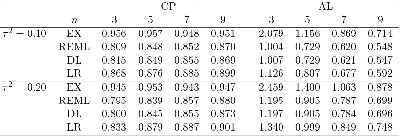
intervals. The results, shown in Table 1, indicate that the confidence intervals from
the three methods other than EX are too liberal to achieve the appropriate nominal
level 0.95 even whenn= 9. On the other hand, the EX method produces reasonable
confidence intervals with appropriate coverage probabilities even when nis 3.
Table 1: Simulated coverage probabilities (CP) and average lengths (AL) of 95% confidence intervals from the proposed exact (EX) method, the restricted maximum likelihood (REML) method, the DirSimonian and Laird (DL) method, and the like-lihood ratio (LR) method.
CP AL
n 3 5 7 9 3 5 7 9
τ2= 0.10 EX 0.956 0.957 0.948 0.951 2.079 1.156 0.869 0.714
REML 0.809 0.848 0.852 0.870 1.004 0.729 0.620 0.548
DL 0.815 0.849 0.855 0.869 1.007 0.729 0.621 0.547
LR 0.868 0.876 0.885 0.899 1.126 0.807 0.677 0.592
τ2= 0.20 EX 0.945 0.953 0.943 0.947 2.459 1.400 1.063 0.878
REML 0.795 0.839 0.857 0.880 1.195 0.905 0.787 0.699
DL 0.800 0.845 0.855 0.873 1.197 0.905 0.784 0.696
LR 0.833 0.879 0.887 0.901 1.340 0.999 0.849 0.748
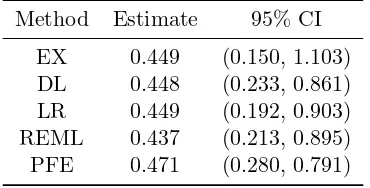
3.4 Example: treatment of suspected acute myocardial infarction
Here we applied the proposed method to a meta-analysis of the treatment of suspected
acute myocardial infarction with intravenous magnesium (Teo et al., 1991), which is
well-known as it yielded conflicting results between meta-analyses and large clinical
trials (LeLorier et al., 1997). For the dataset, we constructed a 95% confidence
EX method (with 10000 Monte Carlo samples in evaluating thep-value) as well as the
REML, DL and LR methods considered in the previous section. Moreover, we also
applied Peto’s fixed effect (PFE) method (Yusuf, 1985). The results are given in Table
2. The confidence intervals from the DL, LR, REML, and PFE methods were narrower
than that of the EX method since the first four methods cannot adequately account
for the additional variability in estimating the between study varianceτ2. Therefore,
the confidence intervals from the first four methods did not coverµ= 1, which does
not change the interpretation of the results. On the other hand, the proposed EX
method produced a longer confidence interval than the other four methods while also
coveringµ = 1, that is, the corresponding test for µ = 1 was not significant with a
5% significant level.
Table 2: Estimates and confidence intervals of the average treatment effect of intra-venous magnesium on myocardial infarction based on six methods.
Method Estimate 95% CI
EX 0.449 (0.150, 1.103)
DL 0.448 (0.233, 0.861)
LR 0.449 (0.192, 0.903)
REML 0.437 (0.213, 0.895)
PFE 0.471 (0.280, 0.791)
4 Bivariate Meta-analysis of Diagnostic Test Accuracy
4.1 Bivariate random-effects model
There has been increasing interest in systematic reviews and meta-analyses of data
from diagnostic accuracy studies. For this purpose, a bivariate random-effect model
(Reitsma et al., 2005 and Harbord et al., 2007) is widely used. Following Reitsma et al.
(2005), we defineµAiandµBi as the logit-transformed true sensitivity and specificity,
bivariate normal distribution:
where µA and µB are the average logit-transformed sensitivity and specificity, and
σA(>0) and σB(>0) are standard deviations ofµAi and µBi, respectively. Here the
parameterρ∈(−1,1) allows correlation betweenµAi andµBi. The unknown
param-eters are µA, µB, σA2, σB2 and ρ. Let yAi and yBi be the observed logit-transformed
sensitivity and specificity, and we assume that
be more valuable than separate confidence intervals since sensitivity and specificity
might be highly correlated. Reitsma et al. (2005) suggested the 100(1−α)% joint
CR forµas the interior points of the ellipse defined as
µA=µbA+cαsbAcost, µB =µbB+cαbsBcos(t+ arccosρb), t∈[0,2π), (8)
where µbA and µbB are the maximum likelihood estimates of µA and µB, bsA and bsB
are estimated standard errors of µbA and µbB, respectively, and cα is the square root
of the upper 100α% point of theχ2 distribution with 2 degrees of freedom. The joint
CR (8) is approximately valid; specifically, the coverage error converges to 1−α as
the number of studies n goes to infinity. However, when n is not sufficiently large,
the coverage error is not negligible, and the region (8) undercovers the trueµ.
4.2 Exact CR of sensitivity and specificity
We consider an exact CR ofµunder the models (6) and (7) based on the Monte Carlo
method given in Section 2. Letψ= (σA2, σB2, ρ)t be a vector of nuisance parameters,
LRT statistic of the null hypothesis H0:µ=µ0 is given by
Under H0, the constrained maximum likelihood estimatorψbcsatisfies the following
equations:
solution can be numerically obtained by minimizing the sum of squared values of
three equations with respect toψ. Moreover, concerning the weight (2), we may use
the numerical derivative given U. Hence, we can compute the exact p-value of the
LRT of H0:µ=µ0 from Algorithm 1.
From the LRT of H0, the (1−α)% exact CR of µ can be defined as ECRα =
{µ;p(µ)≥α}, wherep(µ) denotes the exactp-value of the test statisticTµ(Y). Since
µ is two-dimensional in this case, the computing boundary {µ;p(µ) = α} is not
sufficiently large numbers of points. To this end, we first divide the interval [0,2π) by
M points 0 =t1 <· · ·< tM <2π. For eachm= 1, . . . , M, we computerm satisfying
p(µb+ (rmcostm, rmsintm)) =α,
which can be carried out via numerical methods (e.g. the bisectional method).
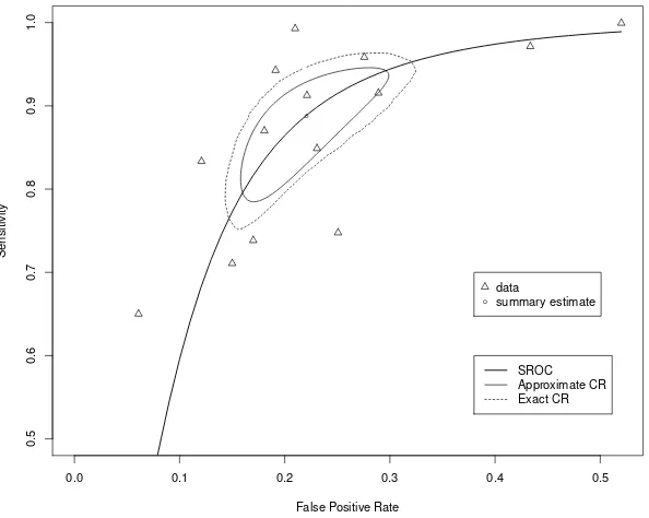
4.3 Example: screening test accuracy for alcohol problems
Here we provide a re-analysis of the dataset given in Kriston et al. (2008), including
n = 14 studies regarding a short screening test for alcohol problems. Following
Reitsuma et al. (2005), we used logit-transformed values of sensitivity and specificity,
denoted byyAiandyBi, respectively, and associated standard errorssAiandsBi. For
the bivariate summary data, we fitted the bivariate models (6) and (7), and computed
95% CRs of µ based on the approximated CR of the form (8) given in Reitsma
et al. (2005). Moreover, we computed the proposed exact CR with 1000 Monte
Carlo samples for calculating p-values of the LRT, and M = 200 evaluation points
that were smoothed by a 7-point moving average for the CR boundary. Following
Reitsuma et al. (2005), the obtained two CRs of (µA, µB) were transformed to the
scale (logit(µA),1−logit(µB)), where logit(µA) and 1−logit(µB) are the sensitivity
and false positive rate, respectively. The obtained two CRs are presented in Figure
1 with a plot of the observed data, summary points bµ, and the summary receiver
operating curve. The approximate CR is smaller than the exact CR, which may
indicate that the approximation method underestimates the variability of estimating
nuisance variance parameters.
5 Network Meta-analysis
5.1 Multivariate random-effects model
Suppose there are p treatments in contract to a reference treatment, and let yir be
0.0 0.1 0.2 0.3 0.4 0.5
0.5
0.6
0.7
0.8
0.9
1.0
False Positive Rate
Sensitivity
●
●
data
summary estimate
SROC Approximate CR Exact CR
Figure 1: Approximated and exact confidence regions (CRs) and summary receiver operating characteristics (SROC) curve.
consider the following multivariate random-effects model:
yi ∼N(θi, Si), θi ∼N(β,Σ), i= 1, . . . , n. (9)
where yi = (yi1, . . . , yip)t, θi = (θi1, . . . , θip)t is a vector of true treatment effects in
the ith study, β = (β1, . . . , βp)t is a vector of average treatment effects, and Si is
the within-study variance-covariance matrix. Here we focus on the model (9) known
as the contrast-based model (Salanti et al., 2008; Dias and Ades, 2016), which is
commonly used in practice.
In network meta-analysis, each study contains onlypi(< p) treatments (pi usually
ranges from 2 to 5); thereby, several components in yi cannot be defined. When
the corresponding treatments are not involved in the ith study, the corresponding
components in yi and Si are shrunk to the sub-vector and sub-matrix, respectively,
in the model (9). Moreover, when the references treatment is not involved in theith
a quasi-small data set is added to the reference arm, e.g. 0.001 events for 0.01 patients.
To clarify the setting in whichyiandSi are shrunk to the sub-vector and sub-matrix,
respectively, we introduce an index aij ∈ {1, . . . , p}, j = 1, . . . , pi, representing the
treatment estimates that are available in theith study, and define the p-dimensional
vectorxij of 0’s, excluding theaijth element that is equal to 1. Moreover, we define
Xi = (xi1, . . . , xipi)
t, andy
i andSi are the shrunkenpi-dimensional vector andpi×pi
matrix ofyi and Si, respectively. The model (9) can be rewritten as
yi∼N(Xiθi, Si), θi ∼N(β,Σ), i= 1, . . . , n. (10)
Regarding the structure of between study variance Σ, since there are rarely enough
studies to identify the unstructured model of Σ, the compound symmetry structure
Σ = τ2P(0.5) is used in most cases (White, 2015), where P(ρ) is a matrix with all
diagonal elements equal to 1 and all off-diagonal elements equal toρ.
We define y = (yt1, . . . , ynt)t, X = (X1t, . . . , Xnt)t, Z = diag(X1, . . . , Xn), and
u= (ut
1, . . . , utn)twithui∼N(0, τ2P(0.5)) independently for eachi. The hierarchical
model (10) can be expressed as the following random-effects model:
y=Xβ+Zu+ε, (11)
whereε∼N(0, S) with S = diag(S1, . . . , Sn). The unknown parameters in (11) are
β and τ2. The log-likelihood of the model (11) is given by
L(β, τ2) =−1
2log|V(τ
2)
| −12(y−Xβ)tV(τ2)−1(y−Xβ),
whereV(τ2) =τ2Z{In⊗P(0.5)}Zt+S and ⊗denotes the Kronecker product. Note
thaty is anN-dimensional vector and N =PnI=1pi is the total number of
5.2 Exact confidence interval of the average treatment effect
In network meta-analysis, we are interested in not only the average treatment effects
β1, . . . , βp in contrast to the reference treatment, but also the treatment differences
βj −βk, j 6= k. To handle these issues in a unified manner, we focus on the linear
combination η = ctβ with known vector c. Define a full-rank p×p matrix A such
that the first element of Aβ is η. The parameter η is equivalent to β1 when we use
XA−1 instead ofXin the model (11), so that it is sufficient to consider an exact test
and confidence interval ofβ1.
DefineW1 andW2 to beN×1 andN×(p−1) matrices such thatX= (W1, W2),
andω = (β2, . . . , βp)t. The model (11) can be rewritten as
y=W1β1+W2ω+Zu+ε. (12)
We first consider testing of H0 :β1=β10, noting that ω and τ2 are nuisance
param-eters. The LRT statistics can be defined as
Tβ10(Y) = min
β1,ω,τ2
L(β1, ω, τ2)−min
ω,τ2L(β10, ω, τ
2),
where
L(β1, ω, τ2) = log|V(τ2)|+ (y−W1β1−W2ω)tV(τ2)−1(y−W1β1−W2ω).
Under H0, the constrained maximum likelihood estimator ωbc and τbc2 satisfy the
fol-lowing equations:
W2tV(τbc2)−1r(β10,ωbc) = 0
trV(τbc2)−1Q −r(β10,bωc)tV(τbc2)−1QV(τbc2)−1r(β10,ωbc) = 0,
(13)
ofV(τ2) such thatA(τ2)A(τ2)t=V(τ2). The equation (13) can be rewritten as
solution of the above equation with respect to τ2. Hence, the solutions of (14) with
respect toω and τ2 are given byω∗(u) =ω∗(u, τ∗2(u)) andτ∗2(u), respectively.
Con-cerning the weight functionw(U), from the implicit function theorem, it follows that
w(U) =
On the other hand, because derivation of analytical expressions of the partial
deriva-tives with respect to τ2 or bτc2 requires tedious algebraic calculation, we can use
compute the exactp-value of LRT, and the exact confidence interval can be obtained
as well by inverting the LRT.
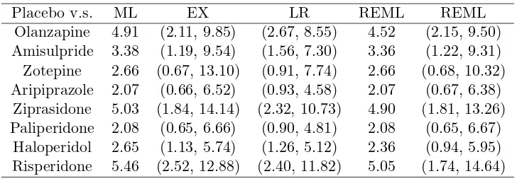
5.3 Example: Schizophrenia data
Ades et al. (2010) carried out a network meta-analysis of antipsychotic medication
for prevention of relapse of schizophrenia; this analysis includes 15 trials comparing
eight treatments with placebo. In each trial, the outcomes available were the four
outcome states at the end of follow-up: relapse, discontinuation of treatment due to
intolerable side effects and other reasons, not reaching any of the three endpoints,
and still in remission. We here considered the last outcome and adopted the odds
ratio as the treatment effect measure.
We applied the multivariate random-effects model (11) with a compound
symme-try structure of Σ. The reference treatment was set to “Placebo”. The estimates of
between-studies standard deviation τ were 0.28 for the ML and 0.52 for the REML
estimation methods, respectively, which shows that there is substantial heterogeneity
between studies.
In Table 3 we present the results of three confidence intervals based on the EX
method, the LR-based method withp-value calculated by the asymptotic distribution,
and the REML method. The number of Monte Carlo samples in applying the EX
method was consistently set to 20000. In this analysis, the confidence intervals of
the EX method were much wider than those of the LR method, and indicated larger
uncertainty in the inference of average treatment effects. On the other hand, the
confidence intervals of the REML method were wider than those of the EX method
in the last three treatments although the REML method produced narrower intervals
than the EX method in the first five treatments; this may be due to the difference
between the ML and REML estimates of between study standard deviation (0.28 for
Table 3: Maximum likelihood (ML) and restricted maximum likelihood (REML) estimates of average treatment effects and confidence intervals from exact (EX), like-lihood ratio (LR) and REML methods in the application to network-meta analysis of schizophrenia data.
Placebo v.s. ML EX LR REML REML
Olanzapine 4.91 (2.11, 9.85) (2.67, 8.55) 4.52 (2.15, 9.50) Amisulpride 3.38 (1.19, 9.54) (1.56, 7.30) 3.36 (1.22, 9.31) Zotepine 2.66 (0.67, 13.10) (0.91, 7.74) 2.66 (0.68, 10.32) Aripiprazole 2.07 (0.66, 6.52) (0.93, 4.58) 2.07 (0.67, 6.38)
Ziprasidone 5.03 (1.84, 14.14) (2.32, 10.73) 4.90 (1.81, 13.26) Paliperidone 2.08 (0.65, 6.66) (0.90, 4.81) 2.08 (0.65, 6.67)
Haloperidol 2.65 (1.13, 5.74) (1.26, 5.12) 2.36 (0.94, 5.95) Risperidone 5.46 (2.52, 12.88) (2.40, 11.82) 5.05 (1.74, 14.64)
6 Discussions
We developed an exact method for constructing confidence intervals of the average
treatment effects in random-effects meta-analysis. The proposed confidence interval
is based on the LRT, and we proposed a Monte Carlo method to compute its exact
p-value without using large sample approximation. In terms of specific applications,
we discussed three types of analysis, univariate analysis, diagnostic
meta-analysis, and network meta-meta-analysis, and demonstrated the usefulness of the proposed
method. The developed exact inference method can be adapted to a variety of
ap-plications, e.g., the multivariate individual participant data meta-analysis (Burke et
al., 2016).
Although we considered exact confidence intervals based on the LRT and the
max-imum likelihood estimators for model parameters, other statistical methods might be
adopted in a similar manner to produce exact confidence intervals. For example,
the REML estimator of heterogeneity variance-covariance can be used instead of the
maximum likelihood estimator since the REML estimator is also sufficient statistics
based on the fact that the restricted likelihood can be derived as the marginal
likeli-hood integrated with respect to mean parameters or regression coefficients (Harville,
1974). Moreover, we could adopt other testing procedures, e.g., the Wald test and
because they use the same principle of theoretical justification of exactness.
In addition, the numerical results from our simulations and the illustrative
exam-ples suggest that statistical methods in the random-effects models should be selected
carefully in practice. Historically, there have been many discrepant results between
meta-analyses and subsequent large randomized clinical trials (LeLorier et al, 1997),
and in these cases the meta-analyses have typically tended to provide false results as
in the magnesium example in Section 3.4. Many systematic biases, for example,
pub-lication bias (Begg and Berlin, 1988; Easterbrook et al., 1991), might be important
sources of these discrepancies, but we should also be aware of the risk of providing
overconfident and misleading interpretations caused by the statistical methods based
on large sample approximations. Considering these risks, accurate inference methods
would be preferred in practice. Although there have not been any exact inference
methods that can be broadly applied in random-effects meta-analyses, our approach
in this article may provide an explicit solution to this relevant problem.
Finally, methodological research on extensions of random-effects meta-analyses to
more complicated statistical models are still in progress (e.g., multivariate network
meta-analyses, Riley et al., 2017), and the small sample problems generally exist
in most of these applications. Our methods are applicable to these complicated
models as well as more advanced approaches that might arise in future research.
The developed methods should be effective tools as a unified exact methodological
framework to obtain accurate solutions in medical evidence synthesis.
Acknowledgements
This research was partially supported by CREST (grant number: JPMJCR1412),
JST and JSPS KAKENHI Grant Numbers JP17K19808, JP15K15954, JP16H07406.
References
[1] Ades, A. E., Mavranezouli, I., Dias, S., Welton, N. J., Whittington, C. and
in Health, 13, 976-983.
[2] Begg, C. and Berlin, J. A. (1988). Publication bias: a problem in interpreting
medical data. Journal of the Royal Statistical Society: Series A, 151, 419-463.
[3] Brockwell, S. E. and Gordon, I. R. (2001). A comparison of statistical methods
for meta-analysis.Statistics in Medicine, 20, 825-840.
[4] Brockwell, S. E. and Gordon, I. R. (2007). A simple method for inference on an
overall effect in meta-analysis. Statistics in Medicine, 26, 4531-4543.
[5] Burden, R. L. and Faires, J. D. (2010).Numerical Analysis, 9th Edition,
Brooks-Cole Publishing.
[6] Burke, D. L., Ensor, J. and Riley, R. D. (2016). Meta-analysis using individual
participant data: one-stage and two-stage approaches, and why they may differ.
Statistics in Medicine, 36, 855-875.
[7] DerSimonian, R and Laird, N. M. (1986). Meta-analysis in clinical trials.
Con-trolled Clinical Trials, 7, 177-188.
[8] Dias, S. and Ades, A. E. (2016). Absolute or relative effects? Arm-based
syn-thesis of trial data. Research Synthesis Methods, 7, 23-28.
[9] Easterbrook, P. J., Gopalan, R., Berlin, J. A. and Matthews, D. R. (1991).
Publication bias in clinical research. The Lancet, 337, 867-872.
[10] Guolo, A. (2012). Higher-order likelihood inference in analysis and
meta-regression. Statistics in Medicine, 31, 313-327.
[11] Harbord, R. M., Deeks, J. J., Egger, H., Whiting, P. and Sterne. J. A. C.
(2007). A unification of models for meta-analysis of diagnostic accuracy studies.
Biostatistics, 8, 239-251.
[12] Hardy, R. J. and Thompson, S.G. (1996). A likelihood approach to
[13] Harville, D. A. (1974). Bayesian inference for variance components using only
error contrasts. Biometrika, 61, 383-385.
[14] Henmi, M and Copas J. (2010). Confidence intervals for random effects
meta-analysis and robustness to publication bias. Statistics in Medicine, 29,
2969-2983.
[15] Higgins, J. P. T. and Green, S. (2011) Cochrane Handbook for Systematic
Reviews of Interventions, Version 5.1.0 (The Cochrane Collaboration, Oxford).
[16] Jackson, D and Bowden, J. (2009). A re-evaluation of the ‘quantile
approxi-mation method’ for random effects meta-analysis. Statistics in Medicine, 28,
338-348.
[17] Jackson, D. and Riley, R. D. (2014). A refined method for multivariate
meta-analysis and meta-regression. Statistics in Medicine, 33, 541-554.
[18] Kriston, L., H¨oelzel, L., Weiser, A., Berner, M., and Haerter, M. (2008).
Meta-analysis: Are 3 Questions Enough to Detect Unhealthy Alcohol Use? Annals
of Internal Medicine, 149, 879-888.
[19] LeLorier, J., Gregoire, G., Benhaddad, A., Lapierre, J. and Derderian, F.
(1997). Discrepancies between meta-analyses and subsequent large randomized,
controlled trials. The New England Journal of Medicine, 337, 536-542.
[20] Lindqvist, B. H. and Taraldsen, G. (2005). Monte Carlo conditioning on a
sufficient statistic. Biometrika, 92, 451-464.
[21] Lockhart, R. A., O’reilly, F. J. and Stephens, M. A. (2007). Use of the Gibbs
sampler to obtain conditional tests, with applications. Biometrika, 94, 992-998.
[22] Lu, G. and Ades, A. E. (2006). Assessing evidence inconsistency in mixed
treat-ment comparisons. Journal of the American Statistical Association, 101,
[23] Noma, H. (2011). Confidence intervals for a random-effects meta-analysis based
on Bartlett-type corrections. Statistics in Medicine, 30, 3304-3312.
[24] Noma, H., Nagashima, K., Maruo, K., Gosho, M. and Furukawa, T. A. (2017).
Bartlett-type corrections and bootstrap adjustments of likelihood-based
infer-ence methods for network meta-analysis. Statistics in Medicine, to appear.
[25] Reitsma, J. B., Glas, A. S., Rutjes, A. W. S., Scholten, R. J. P. M., Bossuyt, P.
M. and Zwinderman, A. H. (2005). Bivariate analysis of sensitivity and
speci-ficity produces informative summary measures in diagnostic reviews. Journal
of Clinical Epidemiology, 58, 982-90.
[26] Riley, R. D., Jackson, D., Salanti, G., Burke, D. L., Price, M., Kirkham, J.
and White, I. R. (2017). Multivariate and network meta-analysis of multiple
outcomes and multiple treatments: rationale, concepts, and examples BMJ,
358, j3932.
[27] Riley, R. D., Lambert, P. C. and Abo-Zaid, G. (2010). Meta-analysis of
indi-vidual participant data: rationale, conduct, and reporting. BMJ, 340, c221.
[28] Salanti, G. (2012). Indirect and mixed-treatment comparison, network, or
multiple- treatments meta-analysis: many names, many benefits, many
con-cerns for the next generation evidence synthesis tool.Research Synthesis
Meth-ods, 3, 80-97.
[29] Salanti, G, Higgins, J. P., Ades, A. and Ioannidis, J. P. (2008). Evaluation
of networks of randomized trials. Statistical Methods in Medical Research, 17,
279-301.
[30] Sidik, K and Jonkman, J. N. (2002). A simple confidence interval for
meta-analysis.Statistics in Medicine, 21, 3153-3159.
[31] Teo, K. K., Yusuf, S., Collins, R., Held, P. H. and Peto, R. (1991). Effects of
intravenous magnesium in suspected acute myocardial infarction: overview of
[32] White, I. R. (2015). Network meta-analysis.The State Journal, 15, 951-985.
[33] White, I. R., Barrett, J. K., Jackson, D. and Higgins, J. P. T. (2012).
Con-sistency and inconCon-sistency in network meta-analysis: model estimation using
multivariate meta-regression.Research Synthesis Methods, 3, 111-125.
[34] Whitehead, A. and Whitehead, J. (1991). A general parametric approach to
the meta-analysis of randomized clinical trials. Statistics in Medicine, 10,
1665-1677.
[35] Yusuf, S., Peto, R., Lewis, J., Collins, R. and Sleight, P. (1985). Beta blockade
during and after myocardial infarction: an overview of the randomized trials.