Reassessing Accuracy Rates of Median Decisions
Andrea Capotorti,
Frank Lad
and
Giuseppe Sanfilippo
University of Perugia
University of Canterbury
University of Palermo
Key Words: Asbestosis, second opinions, medical diagnosis, specificity, sensitivity, pre-dictive values, coherence, exchangeability, fundamental theorem of prevision, probability bounds, linear programming, quadratic programming
Abstract
We show how Bruno de Finetti’s fundamental theorem of prevision has computable applications in statistical problems that involve only partial information. Specifically, we assess accuracy rates for median decision procedures used in the radiological diagnosis of asbestosis. Conditional exchangeabil-ity of individual radiologists’ diagnoses is recognized as more appropriate than independence which is commonly presumed. The FTP yields coherent bounds on probabilities of interest when available information is insufficient to determine a complete distribution. Further assertions that are natural to the problem motivate a partial ordering of conditional probabilities, extending the computation from a linear to a quadratic programming problem.
1
Introduction
At the invitation of Maurice Fr´echet, Bruno de Finetti (1937) delivered six lectures to the Institute Henri Poincar´e in Paris. In them he showed how probability, and more generally expectation, can be defined in terms of a price, and how the concept of coherence of an array of such prices assessed by an individual generates a unified theory of probability and expectation. He termed the asserted values for observable quantities as “previsions,” and introduced the notation of P(E) and P(X) as common to both assertions. The lectures also introduced the judgment of exchangeability as representing symmetry in one’s uncertain attitudes about a sequence of quantities, implying an inferential procedure for learning about future events in the sequence from the observation of earlier events. The presentation formalized what has been called “de Finetti’s representation theorem” for exchangeable distributions: that infinitely extendible exchangeable assessments of a sequence of events can be represented as mixtures of condition-ally independent distributions. Fincondition-ally, he explained what he later termed “the fundamental theorem of probability” (de Finetti, 1974, Section 3.10) showing how the principle of coherency determines precise and computable bounds on the probability for any event if that probability is to cohere with a list of probabilities and conditional probabilities already specified.
The statistical community today is still coming to grips with the implications of these lectures. They provide a completely different foundation for the prospects and limitations of statistical inference than was the framework in which mainstream statistical theory and practice developed during the twentieth century. The most widely known of de Finetti’s results is his representation theorem for exchangeable distributions. Interpreted as a formulation for how independent random variables can be used for trans-forming a prior distribution for unknown probabilities into a posterior distribution, it is honored by many proponents as a cornerstone for the current practice of Bayesian statistics. Unknown to many statisticians who are familiar with Bayesian computational methods, this is not at all the way de Finetti thought of his mathematical constructions. A sophisticated yet practical introduction to de Finetti’s outlook and statistical methodology appears in the text of Lad (1996).
In the present article, we address an important statistical problem involving multiple radiologists as-sessing the condition of asbestosis in lung tissue by means of X-rays. In doing so, we introduce the basic meaning and relevance of the judgment to regard a sequence of quantities exchangeably, and we show how the fundamental theorem of probability can be used directly in this application to yield computable interval probabilities for the accuracy rates of median diagnoses.
In Section 2 we present summary substantive background for understanding the problem of asbestosis diagnosis. We then present a brief introduction to the meaning of exchangeability in Section 3, and to
the computational use of de Finetti’s fundamental theorem of probability in Section 4. In Section 5 we show how the judgment of conditional exchangeability regarding the assessments of three radiologists, along with some other appropriate judgments, provides inputs for the computation of probability bounds for accuracy rates of “median diagnostic procedures.” Computational results are discussed in Section 6. Throughout the article we use the mathematical syntax and language of de Finetti’s operational-subjective construction of probability and statistical method. TheTASon-line repository contains supplements to the content of Sections 4,5 and 6. More extensive discussion and literature references on all matters can be found in the research report of Capotorti, Lad and Sanfilippo (2003).
2
Accuracy rates of asbestosis diagnosis using three radiologists
The condition of asbestosis (fibrosis of the lung) can be identified precisely only by removing some tissue from a lung and examining it for metallic nodules using histological laboratory procedures. This is con-sidered to be the gold-standard of asbestosis detection. Because there is not much that current medical therapy can do for a patient who has this condition, this histological procedure is seldom undertaken except during autopsies of patients who have died of lung cancer. A cheaper and less invasive, but less precise method of diagnosis is typically followed using lung X-rays. Asbestosis may exhibit itself on an X-ray by a shadowy character to the film. Assessment is so difficult that radiologists must be specially trained to achieve the qualification of a “B-reader” to be permitted to read them. There are graded categories of severity of the condition that can be assessed according to the density of the shadow. Offi-cial standards of the International Labor Organization require that at least two of three speOffi-cialized film readers (each blinded to the assessment of the others) must assess the film in a category “at least as bad as a specified standard” in order for the subject to be recognized as having asbestosis. Such a “median diagnosis” is required in legal proceedings for the award of damages to a worker to be paid by an employer.
We shall designate by F the event that a subject actually has fibrosis of the lung, which could be de-tected by histological examination. The measurementF = 1 denotes the presence of asbestosis detected by such an exam, whileF = 0 denotes no presence. The decisions of the individual radiologists to assign the X-ray to the category of “asbestosis at least as bad as the minimal standard” are denoted as the eventsDi for i = 1, 2, and 3. EachDi= 1 if the ithradiologist makes a positive diagnosis, whileDi= 0
if the diagnosis is negative. Throughout this article we use tilde notation to denote the negation of an event. For example, a negative diagnosis can also be denoted by ˜Di. The median decision, denoted by
D∗, is the event that the sum of the individual diagnosis events is at least 2, i.e.,D∗≡(Σ3
i=1Di≥2).
In any diagnostic problem, there are four conditional probabilities that characterize the accuracy of a physician’s expected diagnostic performance. Specified in terms of an individual radiologist in this problem, these are the probabilities P(Di|F), P(Dei|F˜),P(F|Di), andP( ˜F|Dei). Standard terminology
refers to these probabilities as the sensitivity, specificity, positive predictive value and negative predictive value of a diagnosis. Ideally, all four of these probabilities would be large, as close as possible to 1 in each case. The goal of our analysis is to identify the difference between these characteristic diagnosis probabilities for individual B-readers and the corresponding diagnosis probabilities for the median decision procedure. These are denoted byP(D∗|F),P(De∗|F˜),P(F|D∗), andP( ˜F|De∗). The hope and expectation
is that each of these probabilities would exceed the corresponding accuracy rate of an individual reader’s diagnosis. In the article that originally brought this problem to our attention, Tweedie and Mengersen (1999) estimated the median decision accuracy rates using the assumption that the decisions of the three radiologists are conditionally independent given F and also given ˜F. For reasons that we shall now explain, we propose that the judgment of “conditional exchangeability” is more appropriate to assessments of the mutually blind diagnosis decisions by the three radiologists.
3
Regarding events exchangeably
The stochastic independence of three events is commonly defined by the condition that the probability of joint occurrence of any two or three of them equals the product of their marginal probabilities. This implies thatP(Ei|Ej) =P(Ei) andP(Ei|EjEk) =P(Ei) for any substitution ofi, jand kby 1, 2 or 3.
Consider, for example, the decisions of three radiologists concerning the exhibition of asbestosis on an X-ray. Because the diagnostic judgments of any two of the radiologists are unknown to the third, they could not possibly have had any causal influence on the judgment of the third. According to common conception then, the three diagnosis decisions might well be considered to be independent, and even conditionally independent given F and given ˜F. The state of the X-ray would be considered to cause an individual to make the diagnosis Di or ˜Di, at least probabilistically, not the diagnosis of the other two
readers.
Bruno de Finetti insisted that probabilities are not unobservable properties of nature, but rather representations of individuals’ uncertain assertions about the observable facts of nature. Thus, when considering the difference between, say, an assertion ofP(E2) and an assertion of P(E2|E1) we are not
considering the effect ofE1 onE2, but rather of the information thatconditional knowledgeofE1 would
have onone’s uncertain assessmentof E2. The paradigmatic applications of the concept of “stochastic
independence” to statistical analysis in objectivist thinking involve “random experiments” conducted under “identical conditions.” When probabilities are recognized as the representations of individuals’ uncertainties about events rather than as properties of the events, it is evident that experimental obser-vations of this type arenot regarded independently. Why do we conduct experiments in the first place? We design and conduct them because we are uncertain what is going to happen, and because we would like to learn about what may happen in the later experiments in the sequence from what we observe about the earlier ones. We typically expect to assert different values for P(E2), for P(E2|E1) and for
P(E2|Ef1); and similarly we might assert different values for P(E3) and for P(E3|E1E2), P(E3|E1Ef2),
P(E3|Ef1E2) andP(E3|Ef1Ef2). An interesting condition among these is thatP(E3|E1Ef2) may well equal
P(E3|Ef1E2). We shall pursue this condition further.
One feature of opinions that is common to assessors of such experiments is that the order in which observed successes and failures arriveis regarded as irrelevant to opinions about subsequent results, even among people who may dispute how likely a success may be. It is because the different experiments are conducted in the same way every time that we do not especially expect the successes to come early in the sequence, late in the sequence, or especially alternating. This is the feature that de Finetti characterized as the judgment to regard a sequence of events exchangeably:
Definition: A sequence of N events is regarded exchangeably if the probability for any particular string involving K successes and (N-K) failures is assessed identically, no matter what the order in which the successes and the failures arrive. This must be true for each value of K between 1 and (N-1). ⋄
Agreement to regard the order of successes as irrelevant implies that disagreements among disputants can be reduced by coherent inference from the results of experiments. Three features of exchangeable distributions are especially worth noting.
The assessed probability for any particular ordered string of successes and failures depends only on one’s probability that the sum of the successes equals the sum in that string. Specifically, if N events are regarded exchangeably, then for any permutation of the subscripts on the events denoted by E’s in the following expression, we require the identity
P(E1E2...EKE˜K+1E˜K+2...E˜N) = P(SN =K)/NCK ,
whereSN denotes the sum of the N events. For there areNCK distinct ways to permute the subscripts
and yield a distinct sequence of successes and failures.
If events in a sequence are regarded independently and with identical probabilities (iid), then the sequence is also regarded exchangeably. For in this case, designating the common value of eachP(Ei) by
θ, P(E1E2...EKE˜K+1E˜K+2...E˜N) = θK(1−θ)(N−K) for any permutation of the subscripts. Thus iid
distributions over a sequence of events are exchangeable distributions. However, exchangeable distribu-tions are not necessarily iid. De Finetti’s representation theorem identifies the precise relation between iid distributions and exchangeable distributions. An enjoyable elementary exposition of this theorem appeared in the article of Heath and Sudderth (1976):
Theorem: If a distribution for N events is exchangeable and can be extended to a distribution over any larger number of events as an exchangeable distribution, then for any value of K between 1 and (N-1) and for any permutation of the subscripts on the E’s,
P(E1E2...EKE˜K+1E˜K+2...E˜N) =
R1
0 θ
K(1−θ)(N−K) dF(θ) ,
A misinterpretation of this theorem proposes it as supporting a procedure for “updating a prior distri-bution” for the “true probability” of iid events to a posterior distribution. To the contrary, the usefulness of the theorem is in providing a computational method for sequential forecasting procedures based on the formula it implies forP(EN+1|E1E2...EKE˜K+1E˜K+2...E˜N) for any value of K and for any permutation
of the subscripts. Clearly, the events arenotiid. See Lad (1996, Sections 3.8 - 3.12).
The judgment of exchangeability has direct relevance to assessments of X-rays made by three experts. No one is sure whether an expert reading an X-ray will conclude with a diagnosis D = 1 or D = 0. B-readers’ success rates for diagnosingD= 1 when in factF = 1, and in diagnosing D= 0 whenF = 0 are both unknown; and experts may disagree in their uncertainties about these rates. However, it is widely agreed that uncertain assertions about successful diagnoses must satisfy permutation properties such as
P(D1De2De3|F) = P(De1D2De3|F) = P(De1De2D3|F), and
P(D1D2De3|F) = P(D1De2D3|F) = P(De1D2D3|F).
(1)
Because the three B-readers are regarded as otherwise indistinguishable experts, it is considered that if the patient actually has asbestosis (the condition F) it is just as likely that any one of them makes a diagnosis that dissents from the other two. This is considered true both when one or two of the three make a positive diagnosis. All together, these four equalities represent the judgment of conditional exchangeability about the experts’ diagnoses given F. This is a very important distinction from the judgment of conditional independence, because it recognizes explicitly that the diagnosis by any expert would be informative about the likely diagnoses by the others. Similar equalities of conditional probabilities would pertain when the conditioning event is ˜F as well.
4
The fundamental theorem of probability and its extensions
The fundamental theorem of probability was first described in nugatory form in de Finetti’s Paris lectures, but was named “the fundamental theorem” only in his swan-song text, translated into English in 1974. We describe its working here in a two-part numerical example, which also illustrates how the assertion of exchangeability can be relevant to the solution of a problem. The issue of accuracy rates of median di-agnosis procedures will then provide a real application of the use of the theorem in its most extended form.
Consider two logically independent events,E1andE2. Logical independence means that it is possible
that either, both or neither of these events can occur. LetE3 be the event that occurs only ifE1=E2.
In de Finetti-style notation which recognizes events as numbers, this event is determined arithmetically viaE3= 1 + 2E1E2−E1−E2. Now suppose that information is available to motivate the probability
assertionsP(E1) =.7 andP(E2) =.2. What possible values may be asserted forP(E3) if this probability
is to cohere with the two given probabilities? The computational procedure specified by the FTP for yielding the solution to this problem proceeds as follows, in four steps:
1. Define a column vector of the quantities that are involved in the problem, beginning with the quantities whose prevision is specified as “given” in the problem, and ending with the quantity whose unspecified prevision is under consideration. In this example, this would be the vectorE3≡(E1, E2, E3)T.
2. Make a matrix whose columns list allthe possible observable values of the quantity vector specified in step1. This matrix is called therealmof that vector. Here
R
3. Realize that each of the quantities in the vector defined by step 1 can be expressed as a linear combination of four events that identify the columns of the realm matrix. This would be the vector (Ee1Ee2,Ee1E2, E1Ee2, E1E2)T. The coefficients for these linear combinations are specified in the
corre-sponding rows of the realm matrix defined in equation ( 2). Although probabilities for these four events arenot givenas conditions for the problem, we know that these probabilities must sum to 1 because these events constitute an exclusive and exhaustive partition. Moreover, since the prevision (expectation) of any linear combination of events must equal the same linear combination of the probabilities for those events, and since the probabilities for the first two components of the vectorE3are givenin this problem, we have
We can express them by the matrix equation
P
EE12
1
=
0 0 1 10 1 0 1 1 1 1 1
q4 =
..72
1
(3)
4. Finally, since equation (2) shows thatE3is also a linear function of the partition events, with linear
coefficients specified by the third row of the realm matrix, it must also be true thatP(E3) equals this
linear combination of the incompletely specified vectorq4, viz.,P(E3) = ( 1 0 0 1 )q4.
The four steps of this procedure determine bounds for the probability assertion P(E3) that would
cohere with the conditions given in this problem. They can be computed via two linear programming problems: Find the vectorsq∗
4(min) andq∗4(max) that minimize and maximize ( 1 0 0 1 )q4, respectively,
subject to the three linear conditions on q4 displayed in equation (3). The numerical solution for the
minimum coherent value of P(E3) is .10, corresponding to the vector q∗4(min) = (.1, .2, .7,0)T. The
maximum value forP(E3) is .50, corresponding to q∗4(max) = (.3,0, .5, .2)T.
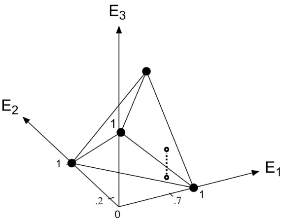
Figure 1 displays the column vectors composing the realm matrix defined in equation (2), each rep-resented by a bold point. The polyhedron that connects them is called their convex hull. A coherent prevision for the vector of unknown quantities (E1, E2, E3)T must be expressible as some convex
combina-tion of these four vertices. Geometrically, this means that the prevision vector must be an interior point or a boundary point of the convex hull. The specification of the first two components ofP(E1, E2, E3)T
as.7 and.2 means further that the vector of all three prevision values must lie on the dashed line segment that touches two edges of the hull in Figure 1. The extreme possibilities forP(E3) correspond to points
on the ends of this line segment.
Figure 1: The convex hull of the column vectors in the realm matrix for (E1, E2, E3)T. The constraintsP(E1) =.7 andP(E2) =.2 restrict the cohering assertion ofP(E3) to lie within limits specified by the endpoints of the dashed line segment touching the boundaries of the convex hull.
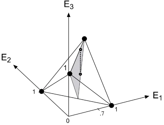
Figure 2 exhibits another interesting application of the FTP, in its more general form as the Fun-damental Theorem of Prevision. Consider the same events composingE3, as above. Now suppose that
the assertion conditions specified in the problem are firstly, that the events E1and E2 are regarded
ex-changeably, and secondly thatP(E1) =.7. Geometrically, the assertion of exchangeability requires that
the prevision vectorP(E3) must lie on the shaded triangular plane displayed in Figure 2. The points on
this plane contain all the triples of P(E3) possibilities for which P(E1Ee2) =P(Ee1E2). Now asserting
this plane whose first two components equal .7. The resulting bounds on P(E3) are determined by the
endpoints of this line segment.
Figure 2: The convex hull of the realm elements is identical to that displayed in Figure 1. Asserting exchangeability ofE1andE2 restricts the coherent prevision vectors to those that lie on the shaded plane. The further assertion ofP(E1) =.7 constrains the limits on a cohering assertion ofP(E3) to the endpoints of the dashed line segment.
Computationally, the conditions of this adjusted problem mean that the constraints on q4 change
from those specified in equation (3) to those in equation (4). The first row constraint onq4 in equation
(4) represents the exchangeability constraint,q2=q3; the second row constraint represents the assertion
P(E1) =.7 ; the third row designates the summation constraint that the components ofq4 sum to 1.
The numerical solution to the modified linear programming problems are that the minimum coherent value of P(E3) is .40, which corresponds to the vectorq∗4(min) = (0, .3, .3, .4)T, while the maximum
value forP(E3) is is 1.0, corresponding toq∗4(max) = (.3,0,0, .7)T.
5
Framing the accuracy of median diagnosis with the FTP
The limited information available in the asbestosis diagnosis problem makes it natural to assess in the format provided by the fundamental theorem of prevision. Neither histological examination of lung tis-sue nor X-ray examination by B-readers is commonly conducted among patients who are not suspected of having asbestosis. Moreover, histological exams are rare even among people who do have asbestosis because of their intrusive nature. However, Tweedie and Mengersen (hereafter T-M, 1999) identified two quantities about which relevant information is available: the frequency of positive median diagnoses among a population of patients who present themselves for asbestosis diagnosis via X-ray; and the fre-quency among such positive diagnoses with which the median diagnosis is determined by a split decision. We designate the event of a positive median diagnosis byD∗, and the event that such a positive diagnosis
arises from a split decision byS∗. The realm for the four basic events along withD∗ andS∗ is
The events relevant to the accuracy rates of median decisions,F andD∗, are both defined in terms of
linear combinations of the partition of events corresponding to the columns ofR. Although information is not available to specify probabilities for each of these columns, information that we can provide does place restrictions on their values:
1. These sixteen probabilities, which we designate in vector notation byq16, must sum to 1.
2. Conditional exchangeability amongD1, D2andD3given F requires thatq6=q7=q8andq12=q13=
q14. For the numerical values ofD1, D2andD3in the associated columns ofRare merely permutations
of one another, and in each of these columns the value ofF = 1. Similarly, exchangeability conditional on ˜F requires thatq3=q4=q5 andq9=q10=q11.
3. Information discussed by T-M motivates assertion values ofP(D∗) =.12 andP(S∗|D∗) =.42.
Equiv-alently for the latter,P(S∗D∗) =.0504.
All together, these assertions amount to eleven linear restrictions on the components ofq16. This leaves
five free dimensions to the specification of q16. We use programming procedures specified by the FTP
to determine bounds on the accuracy probabilities for the median diagnosis procedure that cohere with these input restrictions.
The analysis of T-M involved a stronger assumption, that the individual assessors’ diagnosis decisions are conditionally independent given both F and ˜F. Under these assumptions, the components of q16
could be determined by only three probabilities: P(F), P(Di|F) andP(Dei|F˜). Since these are not di-rectly available, they used the values they assessed forP(D∗) andP(S∗D∗) for two of their inputs, and
then required only a third probability to complete the determination ofq16. The design of their
investi-gation was to propose a range of reasonable possibilities for the unknown value ofP(Di|F) suggested by relevant research literature, and to consider the reasonability of the solutions they imply for the accuracy rates for median decisions. All things considered, their ultimate comparison boiled down to the relative reasonability of two possible assertion values,P(Di|F) =.82 andP(Di|F) =.90.
What we have done is append each of these two assertion possibilities in turn to the eleven restrictions onq16 listed above, and compute the bounds on the median decision accuracy probabilities implied by
the FTP. Before comparing the results, we have one more set of inputs to discuss.
The similar qualifications of the three B-readers support further a partial ordering of conditional probabilities based on their three separate diagnoses, seventeen inequalities in all. We shall display and interpret one array of five inequalities, and then show why they amount to quadratic inequalities condi-tions onq16. A complete presentation of the 17 inequalities is available in the TAS on-line Repository.
Consider the following row of assumed inequalities:
P(D3|Df2Df1Fe) ≤ P(D3|Df1Fe) ≤ P(D3|Fe) ≤P(D3|F) ≤ P(D3|D1F) ≤ P(D3|D2D1F) . (6)
To begin, the middle inequality expresses the view that positive X-ray diagnosis of a patient with fi-brosis is assessed with higher probability than a positive diagnosis for a patient without fifi-brosis. The next inequality to the right expresses the realization that in the context of a patient who has fibrosis, the condition of positive diagnosis by one B-reader motivates a greater expectation of positive diagnosis by the next reader than would be expected without conditioning on the positive diagnosis by the first. Furthermore, a second positive diagnosis would increase our expectation of a positive diagnosis by the third reader even more. This is the content of the final inequality on the right. The inequalities to the left of the central one express the same structure of expectations conditioned on ˜F when we are informed of negative diagnoses.
Now consider for example the first inequality in line (6): P(D3|Df2Df1Fe) ≤ P(D3|Df1Fe). This is an
inequality on two conditional probabilities where the conditioning events are different from one another. Multiplying both sides by the productP(Df2Df1Fe)P(Df1Fe) then yields the equivalent product inequality
P(D3Df2Df1Fe)P(Df1Fe) ≤ P(D3Df1Fe)P(Df2Df1Fe) . (7)
Both multiplicand probabilities on both sides of (7) are expressible as linear functions ofq16. Thus, the
product inequality of line (7) constitutes a quadratic inequality onq16:
Each of the seventeen inequality conditions inserted into our problem induces a quadratic inequality in a similar way. These are referred to as “further inequality conditions” (CondExFIC) in the results of the quadratic programming computations displayed in the next Section.
6
Numerical results
Table 1 contains the computational results of bounds on accuracy probabilities both for individual radi-ologists and for median decisions implied by their coherency with the linear and quadratic conditions we have motivated. To begin their evaluation, notice in comparing column 1 with 2 and column 3 with 4 that the probabilities computed according to the independence assumptions are at or near the endpoints of the intervals allowed by the Conditional Exchangeability assumptions. This is particularly noticeable in the second bank of probabilities relevant to median decisions. This makes sense because the independence assumption entails that the amount of information gained by consulting an additional radiologist (or two) is the maximum possible. Knowledge of the diagnosis of any one radiologist is presumed to provide no information about the diagnosis of any other.
Table 1: BOUNDS ON PROBABILITIES based on the assertions P(D∗) = .12 and P(S∗|D∗) = .42,
along with further assertions appropriate to each column. The first column of numbers displays the T-M probabilities based on the further assertions of conditional independence andP(Di|F) =.82. The second column, labeled CondExFIC, presumes the same three numerical probabilities, but presumes instead conditional exchangeability along with the “further inequality conditions” described in Section 5. Results in the next pair of columns are based on the same presumptions as the first two, except that P(Di|F) is specified as .90. Presumptions for the column headed CondExBnd are the same as for columns 2 and 4 except that only interval bounds [.82, .90] are specified for P(Di|F) andP( ˜Di|F˜). The final column of bounds, headed CondExBPlus, presumes one additional condition, thatP(F|Di)≥.50).
Probability T-M CondExFIC T-M CondExFIC CondExBnd CondExBPlus
p=P(Di|F) .82∗ .82∗ .90∗ .90∗ (.82 , .90 ) (.82 , .846)
1−pf=P(Dfi|Fe) .958* (.797, .992) .894* (.797, .956) (.82 , .90 ) (.898, .90 )
P V+ind=P(F|Di) .734 (.000, .932) .466 (.000, .657) (.000, .506) (.50 , .506)
P V−ind=P(Fe|Dfi) .974 (.973, 1.00) .989 (.988, 1.00) (.975, 1.00) (.975, .981)
P(D∗|F) .914 (.820, .915) .972 (.900, .972) (.82 , .972) (.852, .898)
P(Df∗|Fe) .995 (.880, .995) .968 (.880, .969) (.880, .972) (.969, .972)
P V+ =P(F|D∗) .961* (.000, .961) .761∗ (.000, .762) (.000, .793) (.772, .793)
P V−=P(Fe|Df∗) .987* (.979, 1.00) .997* (.990, 1.00) (.979, 1.00) (.981, .988)
P(F) .126 (.000, .127) .094 (.000, .094) (.000, .111) (.105, .111)
Some of the targeted probabilities of interest are bounded rather tightly by conditional exchange-ability and the further inequality conditions, while others are not. The CondExFIC columns 2 and 4 (entailing p = .82 and p = .90) show fairly tight and nearly equivalent ranges for cohering assertions of the negative predictive valuesP V−ind and the medianP V−; and nearly equivalent and broader but still useable intervals for both individual and median specificitiesP(Dfi|Fe) and P(Df∗|Fe). However, the
ranges for positive predictive valuesP(F|Di) andP(F|D∗) are very broad. Upper bounds differ by .275
and .199 when individual and median diagnoses are compared at the specifications ofp=.82 andp=.90.
One of the uses of bounding results for a wide array of relevant probabilities is to identify further conditions that would help to narrow our focus on important probabilities of interest. One such condition arises from the allowable bounds on the individual radiologists’ positive predictive value,P V+ind. Both
you would rather bet onF, you would want to boundP V+ind above .5. We have conferred with a very
experienced clinical and research oncologist who confirmed that this would be a minimal requirement of assessment probabilities, agreed by virtually every knowledgeable oncologist. It is worth noticing in this regard that the value ofP V+ind implied in the T-M(p=.9) analysis is .466, based on their conditional
independence assumption. Yet the upper bound onP V+indthat coheres with this sensitivity value is as
high as .657 if only conditional exchangeability is presumed. Assuming only conditional exchangeability would free the assessment of all accuracy probabilities to allow sensible ranges.
T-M evaluated their array of implied probabilities in a limited way by questioning the plausibility “that the true positive rate [of an individual diagnosis] should be as low as .82 reported in Kipen et al (1987) since this implies the true negative rate is extremely high” (T-M, 1999, p. 237). They were alluding to the implied probability 1−pf =.958 in the T-M(p=.82) column. However, the lower bound
allowable under exchangeability is as low as .797 in this case (the same as the lower bound implied by their suggested choice ofp=.90). In their discussion of the situation, T-M suggest that perhaps sensi-tivity and specificity might be presumed to be about equal, a feature that further motivated the choice ofp=.9 in their subsequent analysis.
We have followed this thread of T-M’s suggestion in the following way. The fifth column of numer-ical results, headed CondExBnd, again presumes the probabilities P(D∗) = .12 and P(S∗|D∗) = .42
along with the conditional exchangeability of the individual radiologists’ Di given F and ˜F. Rather
than specifying an exact probability for P(Di|F), we merely assert a bound that both probabilities
P(Di|F) andP(Dfi|F˜) must lie within the interval [.82, .90] to represent our uncertainty. As might be expected, most of the probability bounds appearing in this column virtually cover the intersection of the bounds specified in the CondExFIC columns withp=.82 and p=.90. The only really noticeable exceptions occur for the predictive probabilities P(F|Di) and P(F|D∗). The former is now bounded
within the interval (.000, .506) and the latter within (.000, .793). In particular, the interval restrictions onP(Di|F) andP(Dfi|F˜) rule out the higher end of the range on these probabilities allowed whenp=.82.
In the sixth and final column we add the further restriction that the positive predictive value for an individual B-reader should at least exceed .50. The consequences of adding this reasonable assumption are rather severe and illuminating. In the first place, the sensitivity probabilityP(Di|F) is now bounded well away from .90, rather within the fairly tight interval (.82, .846). Moreover, the specificity probability for an individual B-reader,P(Dfi|F˜), is now bounded tightly as well, within the interval (.898, .90). This rules out the higher probabilities that the specification ofp=.82 allows and narrows the interval virtually to equal the value that had been preferred by T-M, motivating their choice ofp=.9 in the context of presumed independence. At the same time, coherency forces the value ofp much closer to .82 than to .9. In fact, all of the accuracy probabilities displayed in the final column compare quite reasonably with the values proposed in the T-M(p = .9) column except for the values of p = .9 and P V+ind = .466.
Moreover, the values they assessed for medianP V−, which might well have been regarded as too high, are tempered a bit, while their unduly low positive predictive values are boosted somewhat. In sum, the assertion of conditional exchangeability supports an assertion ofP(Di|F) around.82 rather than.9. The realism of assumptions allowed by de Finetti’s FTP are critical to understanding this result.
A complete discussion of many related computations is beyond the scope of this article. More details appear in the research report of Capotorti, Lad and Sanfilippo (2003). This includes a commentary on the GAMS computing software which was used for our computational results. See Brooke et al. (2003).
References
Brooke, A., Kendrick, D., Meeraus, A. and Raman, R.(2003)GAMS: a User’s Guide, Washing-ton, D.C.: GAMS Development Corp.
Capotorti, A., Lad, F., and Sanfilippo, G. (2003) Reassessing accuracy rates of median decision procedures, University of Canterbury Department of Mathematics and Statistics Research Report, DMS 2003/21, www.math.canterbury.ac.nz/php/research/reports.
de Finetti, B. Theory of Probability: a critical introductory treatment (1974,1975) 2 volumes, A.F.M. Smith and A. Machi (trs.), New York: Wiley. Translation ofTeoria della probabilita: sintesi introduttiva con appendice critica(1970) Torino: Einaudi.
Heath, D. and Sudderth, W.(1976) De Finetti’s theorem for exchangeable random variables,Amer. Stat., 30, 188-189.
Lad, F.(1996) Operational Subjective Statistical Methods: a mathematical, philosophical, and historical introduction, New York: John Wiley.
Kipen, H.M., Lilis, R., Suzuki, Y., Valciukas, J.A., and Selikoff, I.J.(1987) Pulmonary fibrosis in asbestos insulation workers with lung cancer: a radiological and histopathological evaluation, Brit. Journ. Indust. Med.,44, 96-100.
Materials Associated with this Article
We have prepared three sections of extensions to sections of our article that are necessary for a com-plete statement of precisely how we have made the computations. For much more extensive discussion of all results and even more results, please consult the research report of Capotorti, Lad and Sanfilippo (2003) which is referenced in the article itself.
Appendix 1: Extensions to the four-step computational
procedure appropriate to the most general form of the FTP
We generalize the formal introduction to the FTP here by merely stating some extensions to the four step procedure that are prescribed in its most general form. For details you may consult a reference such as Lad (1996). Any number of previsions or prevision inequalities may be asserted as conditions for the theorem, and the number of constituents in the relevant partition will depend on the number of quantities involved and on the extent of the logical relations among them.
a. References to “events” in the procedure can be replaced by “quantities” and corresponding references to probabilities can be replaced by the unifying concept of “prevision.”
b. Conditional previsions can be included among the assertions given in the suppositions of the theorem, and these will imply linear constraints on the relevant vectorq.
c. Prevision orderings (inequalities) and intervals for previsions may be included among the conditions without affecting the linearity structure.
d. Orderings of conditional previsions that involve different conditioning events are allowable too. How-ever, the constraints these imply onqwould be quadratic rather than linear. (We briefly discussed why this is the case in the asbestosis diagnosis problem.)
e. The object of the enquiry assessed in the theorem can be a conditional prevision too, without affecting the linear structure of the objective function. However, an appropriate transformation of the problem is required to change the ostensibly rational (fractional) objective function into a linear function.
Appendix 2: Twelve more inequalities involving Conditional
Probabilities that were assumed in the computational results
headed “CondexFIC”
The next four rows of inequalities shall be presented in pairs without discussion. Their motivation is similar to the examples outlined in the text of the article. For now, you are left to interpret them and to assert their reasonability for this analysis yourself. You will find them discussed in the technical report mentioned above.
P(D2|Df1Fe) ≤ P(D2|Df1F) ≤ P(D2|F) and
P(D2|Fe) ≤ P(D2|D1Fe) ≤ P(D2|D1F) ; and (9)
P(D3|Df2Df1F) ≤ P(D3|Df1F) ≤ P(D3|Df1D2F) and
P(D3|Df2D1Fe) ≤ P(D3|D1Fe) ≤ P(D3|D2D1Fe) . (10)
The final row of inequalities is centered by a numerical bound.
P(D3|Df1Fe) ≤ P(D3|Df1D2Fe) ≤.5 ≤ P(D3|Df2D1F) ≤ P(D3|D1F) . (11)
In considering the inequalities around .5, think of a question such as this: if you found a patient who suffers from asbestosis (soF = 1 even if this is unbeknownst to you) and you learned that two B-readers made a positive and negative diagnosis based on an X-ray, would you rather bet $1 on the third B-reader making a positive diagnosis or would you rather bet on your flipping a head with a coin in your pocket? If you would rather bet on a positive diagnosis by the third radiologist, then you conditional probability
Appendix 3: More Numerical bound results
To the editor: For now, we are merely appending the bounds on the differences in accuracy probabilities for individual and median decisions that have been deleted from the previous submitted edition. These shall be supplemented further with bounds on a complete list of relevant probabilities and conditional probabilities before the article goes to press. We are currently in the process of extending the computa-tions and constructing the table.
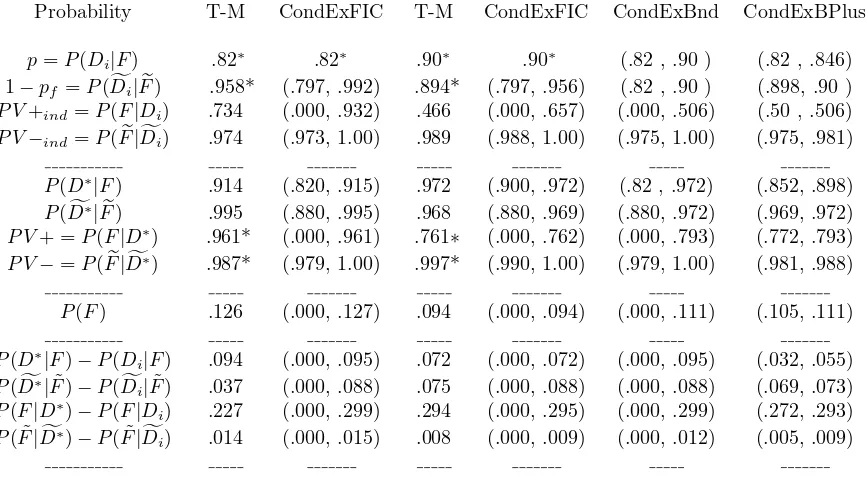
The table below appends to Table 1 shown in the text the bounds on the difference in accuracy probabilities between individual diagnosis decisions and median decisions. The largest gains in accuracy occur in the value of positive predictive values, though gains in sensitivity and specificity of the diagnosis are also of a size that is recognizable. Negative predictive values are already understood to be quite large for the accuracy of individual diagnoses, at least on the order of.975. Thus, absolute gains are not large. Again, as interpreted in the article, the most interesting and sensible of the columns of results is the final one, headed CondExBPlus.
Table 2: FURTHER BOUNDS ON DIFFERENCES IN ACCURACY PROBABILITIES between indi-vidual and median decisions, continuing the assumptions described in the caption to Table 1 of bounds that appear in the article.
Probability T-M CondExFIC T-M CondExFIC CondExBnd CondExBPlus
p=P(Di|F) .82∗ .82∗ .90∗ .90∗ (.82 , .90 ) (.82 , .846)
1−pf =P(Dfi|Fe) .958* (.797, .992) .894* (.797, .956) (.82 , .90 ) (.898, .90 )
P V+ind=P(F|Di) .734 (.000, .932) .466 (.000, .657) (.000, .506) (.50 , .506)
P V−ind=P(Fe|Dfi) .974 (.973, 1.00) .989 (.988, 1.00) (.975, 1.00) (.975, .981)
P(D∗|F) .914 (.820, .915) .972 (.900, .972) (.82 , .972) (.852, .898)
P(Df∗|Fe) .995 (.880, .995) .968 (.880, .969) (.880, .972) (.969, .972)
P V+ =P(F|D∗) .961* (.000, .961) .761∗ (.000, .762) (.000, .793) (.772, .793)
P V−=P(Fe|Df∗) .987* (.979, 1.00) .997* (.990, 1.00) (.979, 1.00) (.981, .988)
P(F) .126 (.000, .127) .094 (.000, .094) (.000, .111) (.105, .111)
P(D∗|F)−P(Di|F) .094 (.000, .095) .072 (.000, .072) (.000, .095) (.032, .055)
P(Df∗|F˜)−P(Dfi|F˜) .037 (.000, .088) .075 (.000, .088) (.000, .088) (.069, .073)
P(F|D∗)−P(F|Di) .227 (.000, .299) .294 (.000, .295) (.000, .299) (.272, .293)