The Physics and Mathematics of Electromagnetic Wave Propagation in Cellular Wireless Communication pdf pdf

The Physics and Mathematics

of Electromagnetic Wave Propagation

in Cellular Wireless Communication

Tapan K. Sarkar

Magdalena Salazar Palma

Mohammad Najib Abdallah

With Contributions from: Arijit De

Walid Mohamed Galal Diab

Miguel Angel Lagunas

Eric L. Mokole

Hongsik Moon

This edition first published 2018 © 2018 John Wiley & Sons, Inc.

All rights reserved. No part of this publication may be reproduced, stored in a retrieval system, or transmitted, in any form or by any means, electronic, mechanical, photocopying, recording or otherwise, except as permitted by law. Advice on how to obtain permission to reuse material from this title is available at http://www.wiley.com/go/permissions.

The right of Tapan K. Sarkar, Magdalena Salazar Palma and Mohammad Najib Abdallah to be identified as the authors of this work has been asserted in accordance with law.

Registered Offices

John Wiley & Sons, Inc., 111 River Street, Hoboken, NJ 07030, USA

Editorial Office

111 River Street, Hoboken, NJ 07030, USA

For details of our global editorial offices, customer services, and more information about Wiley products visit us at www.wiley.com.

Wiley also publishes its books in a variety of electronic formats and by print‐on‐demand. Some content that appears in standard print versions of this book may not be available in other formats.

Limit of Liability/Disclaimer of Warranty

The publisher and the authors make no representations or warranties with respect to the accuracy or completeness of the contents of this work and specifically disclaim all warranties; including without limitation any implied warranties of fitness for a particular purpose. This work is sold with the understanding that the publisher is not engaged in rendering professional services. The advice and strategies contained herein may not be suitable for every situation. In view of on‐going research, equipment modifications, changes in governmental regulations, and the constant flow of information relating to the use of experimental reagents, equipment, and devices, the reader is urged to review and evaluate the information provided in the package insert or instructions for each chemical, piece of equipment, reagent, or device for, among other things, any changes in the instructions or indication of usage and for added warnings and precautions. The fact that an organization or website is referred to in this work as a citation and/or potential source of further information does not mean that the author or the publisher endorses the information the organization or website may provide or recommendations it may make. Further, readers should be aware that websites listed in this work may have changed or disappeared between when this works was written and when it is read.sssss No warranty may be created or extended by any promotional statements for this work. Neither the publisher nor the author shall be liable for any damages arising here from.

Library of Congress Cataloging‐in‐Publication Data

Names: Sarkar, Tapan (Tapan K.), author. | Salazar Palma, Magdalena, author. | Abdallah, Mohammad Najib, 1983– author.

Title: The physics and mathematics of electromagnetic wave propagation in cellular wireless communication / Tapan K. Sarkar, Magdalena Salazar Palma, Mohammad Najib Abdallah ; with contributions from Arijit De, Walid Mohamed Galal Diab, Miguel Angel Lagunas, Eric L. Mokole, Hongsik Moon, Ana I. Perez-Neira.

Description: Hoboken, NJ, USA : Wiley, 2018. | Includes bibliographical references and index. | Identifiers: LCCN 2017054091 (print) | LCCN 2018000589 (ebook) |

ISBN 9781119393139 (pdf ) | ISBN 9781119393122 (epub) | ISBN 9781119393115 (cloth) Subjects: LCSH: Cell phone systems–Antennas–Mathematical models. |

Radio wave propagation–Mathematical models.

Classification: LCC TK6565.A6 (ebook) | LCC TK6565.A6 S25 2018 (print) | DDC 621.3845/6–dc23

LC record available at https://lccn.loc.gov/2017054091 Cover design by Wiley

Cover image: © derrrek/Gettyimages

Set in 10/12pt Warnock by SPi Global, Pondicherry, India

Printed in the United States of America

Contents

Preface xi

Acknowledgments xvii

1 The Mystery of Wave Propagation and Radiation from an Antenna 1

Summary 1

1.1 Historical Overview of Maxwell’s Equations 3 1.2 Review of Maxwell–Hertz–Heaviside Equations 5 1.2.1 Faraday’s Law 5

1.2.2 Generalized Ampère’s Law 8 1.2.3 Gauss’s Law of Electrostatics 9 1.2.4 Gauss’s Law of Magnetostatics 10 1.2.5 Equation of Continuity 11

1.3 Development of Wave Equations 12

1.4 Methodologies for the Solution of the Wave Equations 16 1.5 General Solution of Maxwell’s Equations 19

1.6 Power (Correlation) Versus Reciprocity (Convolution) 24 1.7 Radiation and Reception Properties of a Point Source

Antenna  _{in Frequency and in Time Domain} 28 1.7.1 Radiation of Fields from Point Sources 28

1.7.1.1 Far Field in Frequency Domain of a Point Radiator 29 1.7.1.2 Far Field in Time Domain of a Point Radiator 30 1.7.2 Reception Properties of a Point Receiver 31

1.8 Radiation and Reception Properties of Finite‐Sized Dipole‐Like Structures in Frequencyand in Time 33

1.8.1 Radiation Fields from Wire‐Like Structures in the Frequency Domain 33

1.8.2 Radiation Fields from Wire‐Like Structures in the Time Domain 34 1.8.3 Induced Voltage on a Finite‐Sized Receive Wire‐Like Structure

Due to a Transient Incident Field 34

Contents vi

1.9 An Expose on Channel Capacity 44 1.9.1 Shannon Channel Capacity 47 1.9.2 Gabor Channel Capacity 51

1.9.3 Hartley‐Nyquist‐Tuller Channel Capacity 53 1.10 Conclusion 56

References 57

2 Characterization of Radiating Elements Using Electromagnetic Principles in the Frequency Domain 61

Summary 61

2.1 Field Produced by a Hertzian Dipole 62 2.2 Concept of Near and Far Fields 65

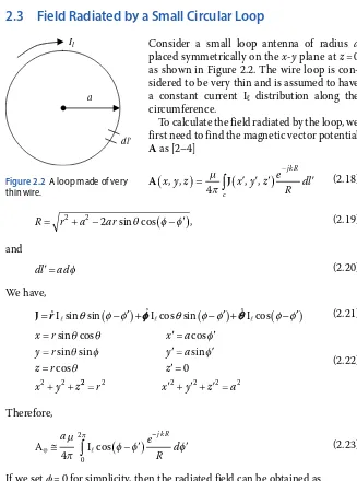
2.3 Field Radiated by a Small Circular Loop 68 2.4 Field Produced by a Finite‐Sized Dipole 70

2.5 Radiation Field from a Finite‐Sized Dipole Antenna 72 2.6 Maximum Power Transfer and Efficiency 74

2.6.1 Maximum Power Transfer 75 2.6.2 Analysis Using Simple Circuits 77

2.6.3 Computed Results Using Realistic Antennas 81 2.6.4 Use/Misuse of the S‐Parameters 84

2.7 Radiation Efficiency of Electrically Small Versus Electrically Large Antenna 85

2.7.1 What is an Electrically Small Antenna (ESA)? 86 2.7.2 Performance of Electrically Small Antenna Versus

Large Resonant Antennas 86

2.8 Challenges in Designing a Matched ESA 90

2.9 Near‐ and Far‐Field Properties of Antennas Deployed Over Earth 94

2.10 Use of Spatial Antenna Diversity 100

2.11 Performance of Antennas Operating Over Ground 104 2.12 Fields Inside a Dielectric Room and a Conducting Box 107 2.13 The Mathematics and Physics of an Antenna Array 120 2.14 Does Use of Multiple Antennas Makes Sense? 123 2.14.1 Is MIMO Really Better than SISO? 132

2.15 Signal Enhancement Methodology Through Adaptivity on Transmit Instead of MIMO 138

2.16 Conclusion 148

Appendix 2A Where Does the Far Field of an Antenna Really Starts Under Different

Environments? 149

Summary 149

2A.1 Introduction 150

2A.2 Derivation of the Formula 2D2/λ ₁₅₃

2A.4 Dipole Antennas Radiating Over an Imperfect Ground 162 2A.5 Epilogue 164

References 167

3 Mechanism of Wireless Propagation: Physics, Mathematics, and Realization 171

Summary 171 3.1 Introduction 172

3.2 Description and Analysis of Measured Data on Propagation Available in the Literature 173

3.3 Electromagnetic Analysis of Propagation Path Loss Using a Macro Model 184

3.4 Accurate Numerical Evaluation of the Fields Near an Earth–Air Interface 190

3.5 Use of the Numerically Accurate Macro Model for Analysis of Okumura et al.’s Measurement Data 192

3.6 Visualization of the Propagation Mechanism 199 3.7 A Note on the Conventional Propagation Models 203

3.8 Refinement of the Macro Model to Take Transmitting Antenna’s Electronic and Mechanical Tilt into Account 207

3.9 Refinement of the Data Collection Mechanism and its Interpretation Through the Definition of the Proper Route 210

3.10 Lessons Learnt: Possible Elimination of Slow Fading and a Better Way to Deploy Base Station Antennas 217

3.10.1 Experimental Measurement Setup 224

3.11 Cellular Wireless Propagation Occurs Through the Zenneck Wave and not Surface Waves 227

3.12 Conclusion 233

Appendix 3A Sommerfeld Formulation for a Vertical Electric DipoleRadiating Over an Imperfect Ground Plane 234

Appendix 3B Asymptotic Evaluation of the Integrals by the Method of Steepest Descent 247

Appendix 3C Asymptotic Evaluation of the Integrals When there Exists a Pole Near the Saddle Point 252

Appendix 3D Evaluation of Fields Near the Interface 254 Appendix 3E Properties of a Zenneck Wave 258

Appendix 3F Properties of a Surface Wave 259 References 261

4 Methodologies for Ultrawideband Distortionless Transmission/ Reception of Power and Information 265

Contents viii

4.2 Transient Responses from Differently Sized Dipoles 268 4.3 A Travelling Wave Antenna 276

4.4 UWB Input Pulse Exciting a Dipole of Different Lengths 279 4.5 Time Domain Responses of Some Special Antennas 281 4.5.1 Dipole Antennas 281

4.5.2 Biconical Antennas 292 4.5.3 TEM Horn Antenna 299

4.6 Two Ultrawideband Antennas of Century Bandwidth 305 4.6.1 A Century Bandwidth Bi‐Blade Antenna 306

4.6.2 Cone‐Blade Antenna 310

4.6.3 Impulse Radiating Antenna (IRA) 313

4.7 Experimental Verification of Distortionless Transmission of Ultrawideband Signals 315

4.8 Distortionless Transmission and Reception of Ultrawideband Signals Fitting the FCC Mask 327

4.8.1 Design of a T‐pulse 329

4.8.2 Synthesis of a T‐pulse Fitting the FCC Mask 331 4.8.3 Distortionless Transmission and Reception

of a UWB Pulse Fitting the FCC Mask 332 4.9 Simultaneous Transmission of Information

and Power in Wireless Antennas 338 4.9.1 Introduction 338

4.9.2 Formulation and Optimization of the Various Channel Capacities 342

4.9.2.1 Optimization for the Shannon Channel Capacity 342 4.9.2.2 Optimization for the Gabor Channel Capacity 344 4.9.2.3 Optimization for the Hartley‐Nyquist‐Tuller Channel

Capacity 345

4.9.3 Channel Capacity Simulation of a Frequency Selective Channel Using a Pair of Transmitting and

Receiving Antennas 347

4.9.4 Optimization of Each Channel Capacity Formulation 353 4.10 Effect of Broadband Matching in Simultaneous Information

and Power Transfer 355 4.10.1 Problem Description 357 4.10.1.1 Total Channel Capacity 358 4.10.1.2 Power Delivery 361

4.10.1.3 Limitation on VSWR 361

4.10.2 Design of Matching Networks 362

4.10.2.1 Simplified Real Frequency Technique (SRFT) 362 4.10.2.2 Use of Non‐Foster Matching Networks 366

4.10.3.2 Constraints of VSWR < 3 369 4.10.3.3 Without VSWR Constraint 371 4.10.3.4 Discussions 372

4.10.4 PCB (Printed Circuit Board) Implementation of a Broadband‐ Matched Dipole 373

4.11 Conclusion 376 References 377

xi

Wireless communication is an important area of research these days. However, the promise of wireless communication has not matured as expected. This is because some of the important principles of electromagnetics were not adhered to during system design over the years. Therefore, one of the objectives of this book is to describe and document some of the subtle electromagnetic princi-ples that are often overlooked in designing a cellular wireless system. These involve both physics and mathematics of the concepts used in deploying anten-nas for transmission and reception of electromagnetic signals and selecting the proper methodology out of a plethora of scenarios. The various scenarios are but not limited to: is it better to use an electrically small antenna, a resonant antenna or multiple antennas in a wireless system? However, the fact of the matter as demonstrated in the book is that a single antenna is sufficient if it is properly designed and integrated into the system as was done in the old days of the transistor radios where one could hear broadcasts from the other side of the world using a single small antenna operating at 1 MHz, where an array gain is difficult to achieve!

provided to demonstrate how a distortion free tens of gigahertz bandwidth signal can be transmitted and received to justify this claim. This technique can be achieved by recasting the Friis’s transmission formula (after Danish‐ American radio engineer Harald Trap Friis) to an alternate form which clearly illustrates that if the physics of the transmit and receive antennas are factored in the channel modelling then the path loss can be made independent of fre-quency. The other important point to note is that in deploying an antenna in a real system one should focus on the radiation efficiency of the antenna and not on the maximum power transfer theorem which has resulted in the misuse of the S‐parameters. Also two antennas which possess a century bandwidth (i.e., a 100:1 bandwidth) are also discussed.

The next topic that is addressed in the book is the illustration of the short-comings of a MIMO system from both theoretical and practical aspects in the sense that it is difficult if not impossible to achieve simultaneously several orthogonal modes of transmission with good radiation efficiency. In this con-text, a new deterministic methodology based on the principle of reciprocity is presented to illustrate how a signal can be directed to a desired user and simul-taneously be made to have nulls along the directions of the undesired ones without an explicit characterization of the operational environment. This is accomplished using an embarrassingly simple matrix inversion technique. Since this principle also holds over a band of frequencies, then the characteri-zation of the system at the uplink frequency can be used to implement this methodology in the downlink or vice versa.

Preface xiii experimental data where possible. Finally, it is shown how to reduce the propa-gation loss by deploying the transmitting antenna closer to the ground with a slight vertical tilt – a rotation about the horizontal axis – a very non-intuitive solution. Deployment of base station antennas high above the ground indeed provides a height‐gain in the far field, but in the near field there is actually a height loss. Also, the higher the antenna is over the ground the far field starts further away from the transmitter.

Finally we introduce the concept of simultaneous transfer of information and power. The requirements for these two issues are contradictory in the sense that transmission of information is a function of the bandwidth of the system whereas the power transfer is related to the resonance of the system which is invariably of extremely narrow bandwidth. To this end, the various concepts of channel capacities are presented including those of an American mathemati-cian and electrical engineer Claude Elwood Shannon, a Hungarian‐British electrical engineer and physicist Dennis Gabor, and an American electrical engineer William G. Tuller. It is rather important to note that each one of these methodologies is suitable for a different operational environment. For exam-ple, the Shannon capacity is useful when one is dealing with transmission in the presence of thermal noise and Shannon’s discovery made satellite com-munication possible. The Gabor channel capacity on the other hand is useful when a system is operating in the presence of interfering signals which is not white background noise. And finally the Tuller capacity is useful in a realistic near field noisy environment where the concept of power flow through the Poynting vector is a complex quantity. Since the Tuller capacity is defined in terms of the smallest discernable voltage levels that the first stage of the RF amplifier can handle and is not related to power, the Tuller formula can be and has been used in the design of a practical system. Tuller himself designed and constructed the first private ground to air communication system and it worked in the first trial and provided a transmission rate which was close to the theoretical design. It is also important to point out that in the development of the various properties of channel capacity it makes sense to talk about the rate of transmission only when one is using coding at the RF stage. To Shannon a transmitter was an encoder and not an RF amplifier and similarly the receiver was a decoder! Currently only two systems use coding at RF. One is satellite communication where the satellite is quite far away from the Earth and the other is in Global Positioning System (GPS) where the code is often gigabits long. In some radar systems, often a Barker code (R. H. Barker, “Group Synchronizing of Binary Digital Systems”. Communication Theory. London: Butterworth, pp. 273–287, 1953) is used during transmission. It is also illus-trated how the effect of matching using both conventional and non Foster type devices have an impact on the channel capacity of a system.

that the superposition of power does not apply in electrical engineering. It is either superposition of the voltages or the currents (or electric and magnetic fields). The other concept is that the energy flow in a wire, when we turn on a switch to complete the electrical circuit, does not take place through the flow of electrons. For an alternating current (AC) system the electrons never actu-ally leave the switch but simply move back and forth when an alternating volt-age is applied to excite the circuit and cause an AC current flow. The energy flow is external to the wire where the electric and the magnetic fields reside and they travel at the speed of light in the given dielectric medium carrying the energy from the source to the load. Also, the transmitting and receiving responses of simple antennas both in time and frequency domains are pre-sented to illustrate the various subtleties in their properties. Maxwell also developed and introduced the first statistical law into physics and formulated the concept of ensemble averaging. In this context, the concepts of information and channel capacity are related to the Poynting’s theorem of electromagnetic energy transmission. This introduces the principle of conservation of energy into the domain of signal analysis which is missing in the context of informa-tion theory. The concepts of the various channel capacities are also introduced in this chapter.

Preface xv antennas over a single antenna is examined. This brings us to the topic of a multiple-input-multiple-output (MIMO) system and its performance in com-parison to a single‐input‐single‐output (SISO) is discussed. Finally, an embar-rassingly simple solution based on the principle of reciprocity is presented to illustrate the competitiveness of this simple system in deployment both in terms of radiation efficiency and cost over a MIMO system.

Chapter 3 deals with the characterization of propagation path loss in a cel-lular wireless environment. The presentation starts with a summary of the various experimental results all of which demonstrate that inside a cell the radio wave propagation path loss is 30 dB per decade of distance and out-side the cell it is 40 dB per decade. This is true irrespective of the nature of the ground whether it be rural, urban, suburban or over water. The path loss is also independent of the operating frequency in the cellular band, height of the base station antennas and so on. Measurement data also illustrate the effect of buildings, trees and the like to the propagation path loss is of a second order effect and that the major portion of the path loss is due to the propagation in  space over ground. A theoretical macro model based on the classical Sommerfeld formulation can duplicate the various experimental data carried out by Y. Okumura and coworkers in 1968. This comparison can be made using a theoretical model based on the Sommerfeld formulation without any mas-saging in the details of the environment for transmission and reception. Thus, the experimental data generated by Y. Okumura and co-workers can be dupli-cated using the Sommerfeld theory. It is important to point out that there are also many statistical models but they do not conform to the results of the experimental data available. And based on the analysis using the macro model developed after Sommerfeld’s classic century old analytical formulation, one can also explain the origin of slow fading which is due to the interference between the direct wave from the base station antenna and the reflection of the direct wave from the ground and occurs only in the near field of the transmit-ting antenna. The so called height gain occurs in the far field of a base station antenna deployment which is generally outside the cell of interest and in the near field within the cell there is actually a height loss, if the antenna is deployed high above the ground. It will also be illustrated using both theory and experi-ment that the signal strength within a cell can significantly be improved by lowering the height of the base station antenna towards the ground. Based on the evidences available both from theory and experiment, a novel method will be presented on how to deploy base‐station antennas by lowering them towards the ground and then slightly tilting them towards the sky, which will provide improvement of the signal loss in the near field over current base station antenna deployments.

of frequencies. To this effect two century bandwidth antennas will be presented and their performances described. Then the salient feature of time domain res-ponses of antennas will be outlined. If these subtleties in time domain antenna theory are followed it is possible to transmit gigahertz bandwidth signals over large distances without any distortion. As such, the phase responses of the antennas as a function of frequency are of great interest for wideband applica-tions. Configurations and schematic of two century bandwidth antennas are presented. The radiation and reception properties of various conventional ultrawideband (UWB) antennas in the time domain are shown. Experimental results are provided to verify how to transmit and receive a tens of gigahertz bandwidth waveform without any distortion when propagating through space. It is illustrated how to generate a time limited ultrawideband pulse fitting the Federal Communication Commission (FCC) mask in the frequency domain and describe a transmit/receive system which can deal with such type of pulses without any distortion. Finally, simultaneous transmission of power and infor-mation is also illustrated and shown how their performances can be optimized over a finite band.

xvii

Thanks are due to Ms. Rebecca Noble (Syracuse University) for her expert typing of the manuscript. Grateful acknowledgement is also made to Dr. John S. Asvestas for suggesting ways to improve the readability of the book.

Tapan K. Sarkar (tksarkar@syr.edu) Magdalena Salazar Palma (salazar@tsc.uc3m.es) Mohammad Najib Abdallah (mnabdall@syr.edu) Syracuse, New York

September 2017

The Physics and Mathematics of Electromagnetic Wave Propagation in Cellular Wireless Communication, First Edition. Tapan K. Sarkar, Magdalena Salazar Palma, and Mohammad Najib Abdallah.

© 2018 John Wiley & Sons, Inc. Published 2018 by John Wiley & Sons, Inc.

1

Summary

An antenna is a structure that is made of material bodies that may consist of either conducting or dielectric materials or may be a combination of both. Such a structure should be matched to the source of the electromagnetic energy so that it can radiate or receive the electromagnetic field in an efficient manner. The interesting phenomenon is that an antenna displays selectivity properties not only in the frequency domain but also in the space domain. In the frequency domain an antenna is capable of displaying an external resonance phenomenon where at a particular frequency the current density induced on it can be suffi-ciently significant to cause radiation of electromagnetic fields from that struc-ture. An antenna also possesses a spatial impulse response that is a function of both the azimuth and elevation angles. Thus, an antenna displays spatial selec-tivity as it generates a radiation pattern that can selectively transmit or receive electromagnetic energy along certain spatial directions in the far field as in the near field even a highly directive antenna has essentially an omnidirectional pat-tern with no selectivity. That is the reason researchers have been talking about space division multiple access (SDMA) where one directs a beam along the direction of the desired user but places a null along the direction of the unde-sired user. This has not materialized as we shall see in the next chapter as most of the base station antennas operate in the near field of an antenna. As a receiver of electromagnetic field, an antenna also acts as a spatial sampler of the electro-magnetic fields propagating through space. The voltage induced in the antenna is related to the polarization and the strength of the incident electromagnetic fields. The objective of this chapter is to illustrate how an electromagnetic wave propagates and how an antenna extracts the energy from such a wave. In addi-tion, it will be outlined why the antenna was working properly for the last few decades where one could receive electromagnetic energy from the various parts

The Mystery of Wave Propagation

1 The Mystery of Wave Propagation and Radiation from an Antenna 2

1.1 Historical Overview of Maxwell’s Equations

In the year 1864, James Clerk Maxwell (1831–1879) read his “Dynamical Theory of the Electromagnetic Field” [1] at the Royal Society (London). He observed theoretically that electromagnetic disturbance travels in free space  with the velocity of light [1–7]. He then conjectured that light is a transverse electromagnetic wave by using dimensional analysis [7] as he did not have the boundary conditions to solve the wave equation except in source free regions. In his original theory Maxwell introduced 20 equations involving 20 variables. These equations together expressed mathematically virtually all that was known about electricity and magnetism. Through these equations Maxwell essentially summarized the work of Hans C. Oersted (1777–1851), Karl F. Gauss (1777–1855), André M. Ampère (1775–1836), Michael Faraday (1791–1867), and others, and added his own radical concept of displacement current to complete the theory.

1 The Mystery of Wave Propagation and Radiation from an Antenna 4

Heaviside for the vector form of Maxwell’s equations, it is important to note that Hertz’s 1884 paper [2] provided the Cartesian form of Maxwell’s equa-tions, which also appeared in his later paper of 1890 [3]. Thus, the coordinate forms of the four equations that we use nowadays were first obtained by Hertz [2, 7] in a scalar form in 1885 and then by Heaviside in 1888 in a vector form [9, 10].

It is appropriate to mention here that the importance of Hertz’s theoretical work [2] and its significance appear not to have been fully recognized [5]. In this 1884 paper [2] Hertz started from the older action‐at‐a‐distance theories of electromagnetism and proceeded to obtain Maxwell’s equations in an alter-native way that avoided the mechanical models that Maxwell used originally and formed the basis for all his future contributions to electromagnetism, both theoretical and experimental. In contrast to the 1884 paper where he derived them from first principles, in his 1890 paper [3] Hertz postulated Maxwell’s equations rather than deriving them alternatively. The equations were written in component form rather than in the vector form as was done by Heaviside [10]. This new approaches of Hertz and Heaviside brought unparalleled clarity to Maxwell’s theory. The four equations in vector notation containing the four  electromagnetic field vectors are now commonly known as Maxwell’s equations. However, Einstein referred to them as Maxwell–Hertz–Heaviside equations [6, 7].

Although the idea of electromagnetic waves was hidden in the set of 20 equa-tions proposed by Maxwell, he had in fact said virtually nothing about electro-magnetic waves other than light, nor did he propose any idea to generate such waves electromagnetically. It has been stated [6, Ch. 2, p. 24]: “There is even some reason to think that he [Maxwell] regarded the electrical production of such waves an impossibility.” There is no indication left behind by him that he believed such was even possible. Maxwell did not live to see his prediction confirmed experimentally and his electromagnetic theory fully accepted. The former was confirmed by Hertz’s brilliant experiments, his theory received universal acceptance, and his original equations in a modified form became the language of electromagnetic waves and electromagnetics, due mainly to the efforts of Hertz and Heaviside [7].

his  theory, and one with enormous practical consequences. That relatively long  electromagnetic waves or perhaps light itself, could be generated in the laboratory with ordinary electrical apparatus was unsuspected through most of the 1870’s.”

Maxwell’s predictions and theory were thus confirmed by a set of brilliant experiments conceived and performed by Hertz, who generated, radiated (transmitted), and received (detected) electromagnetic waves of frequencies lower than light. His initial experiment started in 1887, and the decisive paper on the finite velocity of electromagnetic waves in air was published in 1888 [3]. After the 1888 results, Hertz continued his work at higher frequencies, and his later papers proved conclusively the optical properties (reflection, polariza-tion, etc.) of electromagnetic waves and thereby provided unimpeachable confirmation of Maxwell’s theory and predictions. English translation of Hertz’s original publications [8] on experimental and theoretical investigation of electric waves is still a decisive source of the history of electromagnetic waves and Maxwell’s theory. Hertz’s experimental setup and his epoch‐making findings are described in [9].

Maxwell’s ideas and equations were expanded, modified, and made under-standable after his death mainly by the efforts of Heinrich Hertz, George Francis Fitzgerald (1851–1901), Oliver Lodge (1851–1940), and Oliver Heaviside. The last three have been christened as “the Maxwellians” by Heaviside [7, 11].

Next we review the four equations that we use today due to Hertz and Heaviside, which resulted from the reformulation of Maxwell’s original theory. Here in all the expressions we use SI units (Système International d’unités or International System of Units).

1.2 Review of Maxwell–Hertz–Heaviside Equations

The four Maxwell’s equations are among the oldest sets of equations in math-ematical physics, having withstood the erosion and corrosion of time. Even with the advent of relativity, there was no change in their form. We briefly review the derivation of the four equations and illustrate how to solve them analytically [12]. The four equations consist of Faraday’s law, generalized Ampère’s law, generalized Gauss’s law of electrostatics, and Gauss’s law of mag-netostatics, respectively, along with the equation of continuity.

1.2.1 Faraday’s Law

1 The Mystery of Wave Propagation and Radiation from an Antenna 6

that a magnetic field produced by the bar magnet under some special circumstances can indeed generate an electric field to cause the induced voltage in the loop of  wire and there is a connection between the electric and  magnetic fields. This  physical principle was then put in the following mathematical form:

V

t t s

L

m

S

Ei ℓ Bi

d d (1.1)

where: V = voltage induced in the wire loop of length L,

dℓ = differential length vector along the axis of the wire loop, E = electric field along the wire loop,

Φm = magnetic flux linkage with the loop of surface area S,

B = magnetic flux density,

S = surface over which the magnetic flux is integrated (this surface is bounded by the contour of the wire loop),

L = total length of the loop of wire,

• = scalar dot product between two vectors,

ds = differential surface vector normal to the surface.

This is the integral form of Faraday’s law, which implies that this relation-ship is valid over a region. It states that the line integral of the electric field is equivalent to the rate of change of the magnetic flux passing through an open surface S, the contour of which is the path of the line integral. In this chapter, the variables in italic, for example B, indicate that they are func-tions of four variables, x, y, z, t. This consists of three space variables (x, y, z) and a time variable, t. When the vector variable is written as B, it is a func-tion of the three spatial variables (x, y, z) only. This nomenclature between the variables denoted by italic as opposed to roman is used to distinguish their functional dependence on spatial‐temporal variables or spatial varia-bles, respectively.

To extend this relationship to a point located in a space, we now establish the differential form of Faraday’s law by invoking Stokes’ theorem for the electric field. Stokes’ theorem relates the line integral of a vector over a closed contour to a surface integral of the curl of the vector, which is defined as the rate of spatial change of the vector along a direction perpendicular to its orientation (which provides a rotary motion, and hence the term curl was first introduced by Maxwell), so that

Ei ℓ E i

d d

L S

where the curl of a vector in the Cartesian coordinates is defined by intensity along the respective coordinate directions. The surface S is limited by the contour L. ∇ stands for the operator [ (_xˆ∂ ∂/ x)+_yˆ(∂ ∂/ y)+_zˆ(∂ ∂/ z)]. Using (1.2), (1.1) can be expressed as

Ei ℓ E i Bi

d d d

L S S

s

t s (1.4)

If we assume that the surface S does not change with time and in the limit making it shrink to a point, we get Faraday’s law at a point in space and time as

E D

where the constitutive relationships (here ε and μ are assumed to be constant of space and time) between the flux densities and the field intensities are given by

B H 0 rH (1.6a)

D E 0 rE (1.6b)

D is the electric flux density and H is the magnetic field intensity. Here, ε0 and μ0 are the permittivity and permeability of vacuum, respectively, and εr and μr are the relative permittivity and permeability of the medium through which the wave is propagating.

1 The Mystery of Wave Propagation and Radiation from an Antenna 8

1.2.2 Generalized Ampère’s Law

André M. Ampère observed that when a current carrying wire is brought near a magnetic needle, the magnetic needle is deflected in a very specific way determined by the direction of the flow of the current with respect to the mag-netic needle. In this way Ampère established the complementary connection with the magnetic field generated by an electric current created by an electric field that is the result of applying a voltage difference between the two ends of the wire. Ampère first illustrated how to generate a magnetic field using the electric field or current. Ampère’s law can be stated mathematically as

I

L

Hi ℓ

d _(1.7)

where I is the total current encircled by the contour. We call this the general-ized Ampère’s law because we are now using the total current, which includes the displacement current due to Maxwell and the conduction current. The conduction current flows in conductors whereas the displacement currents flow in dielectrics or in material bodies. In principle, Ampère’s law is con-nected strictly with the conduction current. Since we use the term total cur-rent, we use the prefix generalized as it is a sum of both the conduction and displacement currents. Therefore, the line integral of H, the magnetic field intensity along any closed contour L, is equal to the total current flowing through that contour.

To obtain a point form of Ampère’s law, we employ Stokes’ theorem to the magnetic field intensity and integrate the current density J over a surface to obtain

I s s s

S L S S

Jid

Hidℓ H id 1 B id (1.8)

This is the integral form of Ampère’s law, and by shrinking S to a point, one obtains a relationship between the electric current density and the magnetic field intensity at the same point, resulting in

J( , , , )x y z t H( , , , )x y z t (1.9)

addition to an externally applied impressed current density Ji. So in this case we have

J Ji Jc Jd Ji E D H

t

(1.10)

where D is the electric flux density or electric displacement and σ is the electri-cal conductivity of the medium. The conduction current density is given by Ohm’s law, which states that at a point the conduction current density is related to the electric field intensity by

Jc E (1.11)

The displacement current density introduced by Maxwell is defined by

Jd D

t

(1.12)

We are neglecting the convection current density, which is due to the diffusion of the charge density at that point. We consider the impressed current density only as the source of all the electromagnetic fields.

1.2.3 Gauss’s Law of Electrostatics

Karl Friedrich Gauss established the following relation between the total charge enclosed by a surface and the electric flux density or displacement D passing through that surface through the following relationship:

Di

ds Q

S

(1.13) where integration of the electric displacement is carried over a closed surface and is equal to the total charge Q enclosed by that surface S.

We now employ the divergence theorem. This is a relation between the flux of a vector function through a closed surface S and the integral of the diver-gence of the same vector over the volume V enclosed by S. The divergence of a vector is the rate of change of the vector along its orientation. It is given by

Di iD

ds dv

S V

(1.14)

1 The Mystery of Wave Propagation and Radiation from an Antenna

So the divergence (∇•) of a vector represents the spatial rate of change of the

vector along its direction, and hence it is a scalar quantity, whereas the curl defined mathematically by (∇×) of a vector is related to the rate of spatial change of the vector perpendicular to its orientation, which is a vector quantity and so possesses both a magnitude and a direction. All of the three definitions of grad, Div and curl were first introduced by Maxwell.

By applying the divergence theorem to the vector D, we get

Di iD face S. Therefore, if we shrink the volume in (1.16) to a point, we obtain

(

)

(

)

(

)

This implies that the rate change of the electric flux density along its orienta-tion is influenced by the presence of a free charge density only at that point.

1.2.4 Gauss’s Law of Magnetostatics

Gauss’s law of magnetostatics is similar to the law of electrostatics defined in Section 1.2.3. If one uses the closed surface integral for the magnetic flux den-sity B, its integral over a closed surface is equal to zero, as no free magnetic charges occur in nature. Typically, magnetic charges appear as pole pairs. Therefore, we have

Bi

ds 0 (1.18)

From the application of the divergence theorem to (1.18), one obtains

Equivalently in Cartesian coordinates, this becomes

This completes the presentation of the four equations, which are popularly referred to as Maxwell’s equations, which really were developed by Hertz in scalar form and cast by Heaviside into the vector form that we use today. These four equations relate all the spatial‐temporal relationships between the electric and magnetic fields. In addition, we often add the equation of continuity, which is presented next.

1.2.5 Equation of Continuity

Often, the equation of continuity is used in addition to equations (1.18)–(1.21) to relate the impressed current density Ji to the free charge density qv at that point. The equation of continuity states that the total current is related to the  negative of the time derivative of the total charge by the following relationship

I Q

t

(1.22)

By applying the divergence theorem to the current density, we obtain

I s dv

Now shrinking the volume V to a point results in

v

In Cartesian coordinates this becomes

J x y z t

1 The Mystery of Wave Propagation and Radiation from an Antenna 12

1.3 Development of Wave Equations

To obtain the electromagnetic wave equation, which every propagating wave must satisfy, we summarize the laws of Maxwell’s equations developed in the last section. This is necessary to visualize the fundamental properties related to  wave propagation so that it does not lead to any erroneous conclusions! In free space where there are no available sources the Maxwell’s equations can be written as

Now taking the curl of the first two curl equations one obtains

E ( B) E;

Next we use the Laplacian of a vector Π as

(

)

∇×∇×Π=∇ ∇Π − ∇2Π (1.29)

Since the divergence of either E or B in free space is zero (i.e., the first term in the vector identity drops out), one can then obtain

E 2E 0 0 E E

Here c0 is the velocity of light in free space. The spatial and the temporal deriva-tives for E and B constitute the wave equations in free space for an electromag-netic wave and the speed of light in free space is c0 = 2.99 × 108 m/sec.

A general solution to the electromagnetic wave equation is a linear superposi-tion of waves of the form B(x,t) where this function can have any of the two special form as

B x t, f x c t0 F t x c/ 0 . (1.33)

The function f denotes a fixed pattern in x which travels towards the positive x‐direction with a speed c0. This is illustrated in Figure 1.1 where the wave-shape is propagating. The other function F states equivalently the same thing! So that if an observer is located at a point on this function of f, then the observer’s movement will occur at the phase velocity of the waveform.

An electromagnetic wave can be imagined to compose of a propagating transverse wave of oscillating electric (E) and magnetic fields (B). As shown in Figure 1.2 the electromagnetic wave is propagating from left to right (along the x‐axis). The electric field E is along a vertical plane (y‐axis) and the magnetic field B is in a horizontal plane (z‐axis). The electric and the magnetic fields in an electromagnetic propagating wave are always in temporal phase but spa-tially displaced by 90°. The direction of the propagation of the wave is orthogo-nal to the directions of both the electric and the magnetic fields. This is displayed in Figure 1.2.

f

ct

c

x 0

t t =0

Figure 1.1 A general solution of the wave equation.

y

y

z

x

z _x

B c

→

B

→

E

→

E

→

→

c

→

1 The Mystery of Wave Propagation and Radiation from an Antenna 14

A particular solution of (1.30) for the electric field is of the form E = Em sin(k x − ω t) and is illustrated in Figure  1.2. The magnetic field is of a similar form B = Bm sin(k x − ω t) where the subscripts m represents a magni-tude. So that in this case, the ratio Em/Bm = c0 represents the velocity of light in vacuum and Em/Hm = η = 377Ω represents the characteristic impedance of free space. The magnetic field B is perpendicular to the electric field E in the orien-tation and where the vector product E × B is along the direction of the propa-gation of the wave. As illustrated in Figure 1.2 when a wave is propagating in free space as in a wireless communication scenario, the wave shape moves with time and space and hence the location of neither the minimum nor the maxi-mum in both space and time are stationary. In other words the wave pattern changes as a function of time and space as shown in Figure  1.3 so that the location of the maxima and the minima are not fixed. This is the property of an alternating current wave and is not in any way related to fading.

The component solution (1.33) represents a propagating electromagnetic wave in free space. It tells us that both the maximum and the minimum of the wave moves in time and space. Therefore if its value is zero at a particular instant of space and time it may not be zero at the next spatio‐temporal instance. So there is no fading associated with a travelling wave as its property for propagation is that it changes not only its amplitude continuously but also its position of minima and maxima. So there is no stationary point at which the field is always zero. Hence, it is difficult to conceive then how can one attribute the property of fading to such a signal!

ωt= 0 E_x

Z

ω_t=π_/4 ω_t=π_/2

λ

Since the wave equation contains only c02, changing the sign of c0 makes no difference in the final result. In fact, the most general solution of the one‐ dimensional wave equation is the sum of two arbitrary functions, both of which has to be twice differentiable with space and time. This results in the solution

B x t, f x ct x ct (1.34)

holds in general. The first term represents a wave travelling toward positive x, and the second term constitutes an arbitrary wave travelling toward negative x direction. The general solution is the superposition of two such waves both existing at the same time. Although the function f can be and often is a mono-chromatic sine wave, it does not have to be sinusoidal, or even periodic. In practice, f cannot have infinite periodicity because any real electromagnetic wave must always have a finite extent in time and space. As a result, and based on the theory of Fourier decomposition, a real wave must consist of the super-position of an infinite set of sinusoidal frequencies.

When a forward going wave (given by the first term in (1.34)) interacts with a backward going wave or equivalently a reflected wave (given by the second term in (1.34)) then one obtains a standing wave where the position of the maxima and the minima in amplitude does not change as a function of position even though its amplitude changes as a function of time. Hence, it is a wave that oscillates in time but has a stationary spatial dependence. In that case one may encounter locations of zero field strength for all times but for that to occur one has to operate in an environment which has multiple reflections. Reflections from buildings, trees and the like which are located in an open environment, it is most probable that a standing wave does not occur in such circumstances as seen in the Chapter 2 as one is operating in the near field of the transmitting antenna where there are no pattern nulls and the rays are not defined.

1 The Mystery of Wave Propagation and Radiation from an Antenna 16

alternating electric field (over a distance of a few micrometers). For a 60 Hz alternating current, this means that within half a cycle the electrons drift less than 0.2 μm in a copper conductor. In other words, electrons flowing across the contact point in a switch will never actually leave the switch. In contrast to this slow velocity, individual velocity of the electron at room temperature in the absence of an electric field is ~1570 km/sec.

So the energy transmission in an electrical engineering context is due to the propagating electric and the magnetic fields at the velocity of light and is in no way related to the flow of electrons. The electric and the magnetic fields actu-ally exist and propagate outside the structure. This follows directly from Maxwell’s theory and it is this philosophy that revolutionized twentieth cen-tury science.

1.4

Methodologies for the Solution

of the Wave Equations

The wave equation is a differential equation containing both space and time variables and its unique solution can be obtained from the specific boundary conditions for the fields which should be given for the nature of problem at hand. The solution is quite complex when the excitations are arbitrary func-tions of time. However, when the fields are AC, that is when the time variation of the fields is harmonic of time, the mathematical analysis can be simplified by using complex quantities and invoking Euler’s identity which is given by

ej cos jsin (1.35)

where j 1. This relates real sinusoidal functions with the complex expo-nential function. Any AC quantity can be represented by a complex quantity. A scalar quantity is then interpreted according to

v 2V cos t 2 e Vej t (1.36)

where v is called the instantaneous quantity and V = |V | ej α is called the com-plex quantity. The notation ℜe (•)stands for “the real part of”, that is the part not associated with the imaginary part j. It is important to note that the con-vention v 2 m Ve( j t) can also be used, where the notation ℑm (•) stands for “the imaginary part of”. The factor 2 can be omitted if it is desired that |V| be the peak value of v instead of the rms (root mean square) value.

As an example consider the waveform that is being used in power frequencies. If we say the voltage is 110 V at 50 Hz, then v represents a sinusoidal voltage whose amplitude is 110 and the waveform is similar to the one shown in Figure 1.3. Here we are restricting ourselves to the voltage and hence to the propagating electric field. To observe this waveform we need to use an oscil-loscope where the sinusoidal waveform will be displayed illustrating that this voltage waveform changes as a function of time at the location where we are observing the time varying voltage waveform. This in no way implies that the waveform is displaying fading characteristics as its amplitude changes as a function of time. It is a time domain representation and the waveform should change as a function of time in an alternating current waveform. Therefore, for meaningful measurements that illustrate fading, the measurements should always be carried out in the frequency domain displaying the phasor quanti-ties, particularly its magnitude which is generally a rms (root mean square) value and the associated phase. This magnitude and phase characteristics can be measured by a vector voltmeter or by a vector network analyzer and assum-ing that the waveform beassum-ing watched is not modulated. And if this rms value changes with time then it is meaningful to claim that this wave has an ampli-tude that is time dependent — in other words there may be fading. The phasor voltage V can be measured by a vector voltmeter which will display a reading of 110 and the needle of the voltmeter will remain stationary and will not change with time, even though the waveform is alternating. Now if V is chang-ing with time then the vector voltmeter needle position will change with time and this implies that that there is some sort of variation in the amplitude of the waveform. Then this situation can be characterized by a waveform going through a fade. What is termed slow fading in wireless communication is the interference between the various vector components of the fields (both direct and the reflections from the Earth) and not necessarily multipath components of the signal. As discussed in Chapter 2, multipaths are ray representation of the propagation of the signals and this analysis can only be done in the far field of the antenna. This will be addressed in Chapter 2. Therefore the misuse of the term fading in wireless communication comes because of its misinterpretation and misconception of the fundamentals of electrical engineering principles and thus making a wrong association with a phenomenon that occurs in long wave radio communication where the change of the signal amplitude occurs due to its reflection from the ionosphere and the temporal variation of the electrical properties of the ionosphere which takes place over a time period of seconds or even hours and nothing happens at the milliseconds scale!

1 The Mystery of Wave Propagation and Radiation from an Antenna 18

Finally, there is another phenomenon which is wrongly associated with fast fading and that is Doppler. And again it is due to not comprehending the fun-damental physics of the complete problem! The Doppler frequency is the shift in the carrier frequency when the source or the receiver is moving with a finite velocity. If the source/ receiver is moving with a velocity ϑm/sec then the car-rier frequency of the source will display a Doppler shift in frequency of the signal and is given by

f_d 2 Hz (1.37)

where λ is the wavelength of the original frequency. The shift in frequency is either positive or negative depending on whether the source/receiver is mov-ing towards or away from each other. So if the frequency source is movmov-ing at a relative velocity of 360 kM/hour (= 100 m/sec) which is beyond any real move-ment in a wireless communication scenario, but may exist more in one’s dreams or in an euphoric nonconscious state, then the Doppler shift of a 1 GHz carrier frequency will be fd

2 100

0 3. 666Hz. So the Doppler shift is equal to 666 Hz in a carrier frequency of 109 _{Hz when one is moving at 360 km/hour. If one} takes the best crystal oscillator available in the market, its frequency stability can be at best 1 part in a million implying that the carrier frequency of 1 GHz may vary within 109 _{± 10}3 _{Hz. So, if the crystal oscillator of 1 GHz is moving at} 360 km/hour, the Doppler shift in its frequency is only 666 Hz. Thus, the fact of the matter is that a variation of less than 1 kHz in frequency is simply impos-sible to visualize in a 1 GHz carrier. Hence fast fading due to Doppler is at best a mythology!

Another point to be made here is that one can look at the expression of the propagation of a wave either from the time domain or in the frequency domain using phasors. It is not possible to combine them in any way! However one will find phrases like this in some modern text books on wireless communication: “In response to a transmitted sinusoid cos (2πft), we can express the electric far field at time t asE f t r

f f t r c

r

s

Such a representation has no meaning in electrical engineering and one has to be careful in what one reads in many textbooks on wireless communica-tion these days!! In summary, the voltage across an inductor is Ldi t

dt in the temporal domain and in the phasor domain it is jω L I(ω). However, one cannot write it as jω L i(t)‐ this is actually a meaningless expression in electrical engineering

1.5 General Solution of Maxwell’s Equations

Instead of solving the four coupled differential Maxwell’s equations directly dealing with the electric and magnetic fields, we introduce two additional variables A and ψ. Here A is the magnetic vector potential and ψ is the scalar electric potential. The introduction of these two auxiliary variables facilitates the solution of the four coupled differential equations.

We start with the generalized Gauss’s law of magnetostatics, which states that

(

)

∇_{B x y z t, , ,} =₀ (1.38)

Since the divergence of the curl of any vector A is always zero, that is,

(

)

∇ ∇×_{ A x y z t, , ,} =₀ (1.39)

one can always write

B x y z t, , , A x y z t, , , (1.40)

which states that the magnetic flux density can be obtained from the curl of the magnetic vector potential A. So if we can solve for A, we obtain B by a simple differentiation. It is important to note that at this point A is still an unknown quantity. In Cartesian coordinates this relationship

(

, , ,

)

ˆ

(

, , ,

)

ˆ

(

, , ,

)

ˆ

(

, , ,

)

ˆ

ˆ ˆ

x y z

x y z

x y z t B x y z t B x y z t B x y z t

determinant of

x y z

A A A

= + +

 

 

∂ ∂ ∂

 

= _{ }

∂ ∂ ∂

 

 

 

B x y z

1 The Mystery of Wave Propagation and Radiation from an Antenna

Note that if we substitute B from (1.40) into Faraday’s law given by (1.5), we obtain

If the curl of a vector is zero, that vector can always be written in terms of the gradient of a scalar function ψ, as it is always true that the curl of the gradient of a scalar function ψ is always zero, that is,

x y z t, , , 0 (1.44)

The gradient of a vector is defined through

(

)

This states that the electric field at any point in space and time can be given by the time derivative of the magnetic vector potential and the gradient of the scalar electric potential. So we have the solution for both B from (1.40) and (1.41) and E from (1.46) in terms of A and ψ. The problem now is how we solve for A and ψ. Once A and ψ are known, E and B can be obtained through simple differentiation, as in (1.46) and (1.40), respectively.

Next we substitute the solution for both E [using (1.46)] and B [using (1.40)] into Ampère’s law, which is given by (1.10), to obtain

Ji x y z t E x y z t D H

x y z t

t x y z

, , , , , , , , , , , , t (1.47) Since the constitutive relationships are given by (1.6a) and (1.6b) (i.e., D =εE and B = μH), then is assumed to be the lossless free space, and therefore its conductivity is zero. So we are looking for the solution for an electromagnetic wave propagating in a non‐conducting medium. In addition, we use the following vector’s Laplacian:

(

) (

)

∇ ×∇ ×A= ∇ ∇A − ∇ ∇ A (1.49)

By using (1.49) in (1.48), one obtains

(

) (

)

µ µε ψ

Since we have introduced two additional new variables, A and ψ, we can with-out any problem impose a constraint between these two variables or between the two variables of vector and scalar potentials. This can be achieved by set-ting the right‐hand side of the expression in (1.51) equal to zero. This results in

1 The Mystery of Wave Propagation and Radiation from an Antenna 22

which is known as the Lorenz gauge condition [13]. It is important to note that this is not the only constraint that is possible between the two newly introduced variables A and ψ in our solution procedure. This choice which we have made is only a particular assumption, and other choices will yield different forms of the solution of the Maxwell–Hertz –Heaviside equations. Interestingly, Maxwell in his treatise [1] chose the Coulomb gauge [7], which is generally used for the solution of static problems and not for dynamic time varying problems.

Next, we observe that by using (1.52) in (1.51), one obtains

(

∇ ∇

)

−µε∂ = −µ ∂



2

2 i

t A

A J (1.53)

In summary, the solution of Maxwell’s equations starts with the solution of equation (1.53) first, for A, given the impressed current Ji. Then the scalar potential ψ is solved for by using (1.52). Once A and ψ are obtained, the electric and magnetic field intensities are derived from

H 1B 1 A (1.54)

E A

t (1.55)

This completes the solution in the time domain, even though we have not yet provided an explicit form of the solution. We now derive the explicit form of the solution in the frequency domain and from that obtain the time domain representation. We assume the temporal variation of all the fields to be time harmonic in nature, so that

E x y z t, , , E x y z e, , j t (1.56)

B x y z t, , , B x y z e, , j t (1.57)

where ω = 2 π f and f is the frequency (whose unit is Hertz abbreviated as Hz) of the electromagnetic fields. By assuming a time variation of the form ej ω t, we now have an explicit form for the time differentiations, resulting in

t x y z t t x y z e j x y z e

j t

A , , , A , , A , , jj t (1.58)

Therefore, (1.52) and (1.53) are simplified in the frequency domain after elimi-nating the common time variations of ej ω t from both sides to form

E x y z, , j A x y z, , x y z, , (1.60) Furthermore, in the frequency domain (1.52) transforms into

A j 0

In the frequency domain, (1.53) transforms into

2_A 2 _{A J}

i (1.62)

The solution for A in (1.62) can now be written explicitly in an analytical form as illustrated in [14, 15] as

A

c velocity of light in the medium 1 (1.68)

wavelength in the medium (1.69) In summary, first the magnetic vector potential A is solved for in the fre-quency domain given the impressed currents J_i(r) through

A r A

1 The Mystery of Wave Propagation and Radiation from an Antenna 24

In the time domain the equivalent solution for the magnetic vector potential A is then given by the time‐retarded potentials:

A A

It is interesting to note that the time and space variables are now coupled and they are not separable. That is why in the time domain the spatial and temporal responses of an antenna are intimately connected and one needs to look at the complete solution. From the magnetic vector potential we obtain the scalar potential ψ by using (1.52). From the two vector and scalar potentials the elec-tric field intensity E is obtained through (1.55) and the magnetic field intensity H using (1.54).

We now use these expressions to calculate the impulse response of some typical antennas in both the transmit and receive modes of operations. The reason the impulse response of an antenna is different in the transmit mode than in the receive mode is because the reciprocity principle in the time domain contains an integral over time forming a convolution as it is a simple product in the transformed frequency domain. Thus the mathematical form of the reci-procity theorem in the time domain is quite different from its counterpart in the frequency domain. For the former a time integral is involved, whereas for the latter no such integral is involved as it is a simple product. This relationship comes directly from the Fourier transform theory where a convolution in the time domain is translated into a product in the frequency domain. Because of the simple product in the frequency domain reciprocity theorem, the antenna radiation pattern in the transmit mode is equal to the antenna pattern in the receive mode, except for a scale factor. This is discussed next.

1.6 Power (Correlation) Versus Reciprocity

(Convolution)

with the impulse response h(t) due to an applied input x(t) is given by the following integral representing the convolution of x(t) with h(t) symbolically written as x h as

y(t) = h x= h(t–τ) x(τ) dτ . (1.72)

Next, we discuss the context of reciprocity in electromagnetics. In electro-magnetics the reciprocity relationship in general starts with the Lorentz theo-rem. To establish the Lorentz reciprocity theorem, assume that one has a current density J₁ in a volume V bounded by a closed surface S which produces an electric field E₁ and a magnetic field H₁, where all three are periodic func-tions of time with angular frequency ω_{, and in particular they have a time‐} dependence exp(−jω _{t). Suppose that we similarly have a second current source} J₂ at the same frequency ω _{which (by itself ) produces fields} E₂ and H₂. These fields satisfy Maxwell’s equations and therefore

E1 j H1 H1 j E1 J1 (1.73)

E2 j H2 H2 j E2 J2 (1.74)

By expanding ∇ • (_E1 × _H2 − _E2 × _H1) and simultaneous use of Maxwell’s

equations lead to (as explained in [16])

(

) (

)

(

)

(

)

Integrating now both sides over the volume V and using the divergence theorem yields

where n is the unit outward normal to S. This is the Lorentz reciprocity theorem for an isotropic medium. This mathematical expression is sometimes  also termed as reaction in the computational electromagnetics literature [16].

1 The Mystery of Wave Propagation and Radiation from an Antenna 26

coordinate system. Actually, for any surface S which encloses all the sources for the fields the surface integral will be zero. This can be seen if S becomes the surface of a sphere of infinite radius. Hence, the surface integral taken over any closed surface S surrounding all the sources vanishes. When the surface inte-gral vanishes one obtains

=

∫



∫



V V

dV dV

2 1 1 2

E J E J (1.77)

If J1 and J2 are infinitesimal current elements, then =

 

1 2 2 1

E J E J (1.78)

which states that the electric field E₁ produced by J1 has a component along J2

that is equal to the component along J1 of the field radiated by J2 when both J1

and J2 have unit magnitude. This is the form that is essentially used in circuit

analysis called the Rayleigh‐Carson reciprocity theorem except that E and J are replaced by the voltage V and the current I resulting in

V I1 2 V I2 1 (1.79)

Therefore, the principle of superposition can be applied to both the voltage V

and the current I when applying the principle of reciprocity. Next we consider the principle of correlation, which represents power, in general.

Circuit theory describes the excitation of a two terminal element in terms of the voltage V applied between the terminals and the current I into and out of the respective terminals. The power supplied through the terminal is VI*

(where the superscript * implies a complex conjugate). So in an AC circuit the complex power flow needs to have both V and I to compute the power [14–16]. However, for purely resistive circuits the power can be given solely by either the voltage or the current as they are scalar multiple of each other related to the resistance of the component on which the voltage and the currents are deter-mined. So the correlation between the voltage and the current represents power which is VI*. In this case, superposition does not apply and this holds true even for resistive circuits. As an example consider the two simple circuits of Case A and Case B of Figure 1.4 where two different voltages of 6V and 3V are applied across two individual resistor combination producing currents of 2A and 1A in the respective circuits. The power dissipated in the 1Ω resistor

cohesion as illustrated in Case C or may be in phase opposition resulting in Case D. For case C we observe that the currents and the voltages superpose and the resultant power dissipated in the 1 ohm resistor is now 9W and not 4W+1W = 5W. Does that mean we have a power gain over the two cases A and B? No, definitely not as in electrical engineering the power defined through the principle of correlation states that individual powers cannot be superposed but the voltages and the currents can be combined. Now observe in Case D we have phase opposition between the two superposed voltages and here the 3V source is acting as a load on the 6V source, and instead of supplying useful power it is absorbing it. Hence it is extremely important how in practice gen-erators are connected with the appropriate phase even in the DC situation. As is observed in many practical devices sources are generally connected in series and never in parallel. In a parallel connection of the sources, if there is a slight imbalance of the terminal voltages between the two sources then there will be a nonproductive circulating current. This leads to power loss and also not to minimize the situation that this circulating current may even cause one of the sources to heat up and explode!

Now we extend the concept of power flow in such a way that power is now thought to flow throughout space and is not associated only with a flow of current into and out of the terminals. Just as the circuit laws can be combined to describe the flow of power between the circuit elements, so Maxwell’s equa-tions are the basis for a field theoretical view of power flow expressed through the Poynting’s theorem. The complex power density in space is given by the Poynting vector S as E × H*, where the superscript * represents the complex conjugate. When this power density is integrated over a surface with the

2 A