Groupwise independent component decomposition of
EEG data and partial least square analysis
Natasa Kovacevic
a,⁎
and Anthony Randal McIntosh
a,ba
Rotman Research Institute Baycrest Centre 3560 Bathurst Street, Toronto, Ontario, Canada M6A 2E1 b
Department of Psychology, University of Toronto, Toronto
Received 20 July 2006; revised 10 November 2006; accepted 12 January 2007 Available online 27 January 2007
This paper focuses on two methodological developments for analysis of neuroimaging data. The first is the derivation of robust spatiotemporal activity patterns across a group of subjects using a combination of principal component analysis (PCA) and independent component analysis (ICA). In applications to ERP data, the space dimension is typically represented in terms of scalp electrodes. The signal recorded by high density electrode caps is known to be highly correlated due in part to volume conduction. Consequently, this redundancy is also reflected in spatiotemporal patterns characterizing signal differences across experimental conditions. We present an alternative spatial representation and signal compression based on PCA for dimension-ality reduction and ICA conducted across all subjects and conditions simultaneously. The second advancement is the use of partial least squares (PLS) analysis to assess task-dependent changes in the expression of the independent components. In an application to empirical ERP data, we derive an efficient number of independent component maps. Comparative PLS analysis on the independent components versus original electrode data shows that task effects are not only preserved under compression, but also enhanced statistically. © 2007 Elsevier Inc. All rights reserved.
Introduction
PLS is a multivariate technique that has been utilized in a variety of neuroimaging applications including ERP, MEG, fMRI and PET (McIntosh, 2004; Lobaugh et al., 2001; Duzel et al., 2003; Hay et al., 2002; Addis et al., 2004; Itier and Taylor, 2002). One of the main uses of PLS has been in detecting changes in neuroimaging data due to experimental manipulations of cognitive tasks and describing the changes in terms of spatiotemporal patterns. In applications to functional neuroimaging data represent-ing a group of subjects recorded over several conditions, PLS can detect major experimental effects describing differences in signal intensity across conditions, consistently across subjects. The
experimental effects are further characterized in terms of their expression in space and time.
In most ERP analyses, including PLS, space is represented in terms of electrode potentials and time is represented in terms of latency offsets from time-locking events. Electrodes receive a summed signal from simultaneously active brain sources, and as the signal passes through the skull it becomes spatially smeared across electrodes. In this paper we show how to obtain reduced and efficient spatial representation of an ERP signal as an input to PLS. The representation consists of a set of spatial maps capturing major modes of task related activation for a given event related experiment.
Our spatial data reduction is based on PCA dimensionality re-duction followed by ICA rotation. The PCA/ICA analysis is performed across all subject and conditions in order to identify robust spatiotemporal patterns. Many applications of ICA to EEG data extract meaningful components at the individual subject level. Subject-specific components are then combined based on similarity metrics (Makeig et al., 2004). While there is reason to believe that such an approach will yield similar results to the group-based ICA we propose, there is an important assumption behind our approach versus subject-specific ICA. In our derivation, the assumption is that there are enough similarities across individuals in cortical anatomy/ geometry that a group-based metric is a reasonable topographic summary of task-dependent effects. As such, the components we extract can be considered as a set of spatial filters that are optimized to project subject data into a common spatial reference. The approach is similar in concept to that used in fMRI, where data at the subject level are converted to a common spatial reference, and group ana-lyses performed to extract the most reliable effects across the sample (whether through mixed effects or conjunction analysis (Friston et al., 1999) or resampling (e.g.,Strother et al., 2002; McIntosh, 2004)). Group ICA components are fixed scalp maps with mutually independent time courses. They are viewed as a new and reduced coordinate system for the spatial representation of the EEG data. Single trial time series of the group ICA components are calculated as weighted sums of electrode activations. Individual subject average time series (wave forms) of group ICA are calculated by averaging single trial time series. This component based spatio-NeuroImage 35 (2007) 1103–1112
⁎Corresponding author.
E-mail address:[email protected](N. Kovacevic).
Available online on ScienceDirect (www.sciencedirect.com).
temporal data representation is then analyzed with PLS in order to detect and characterize main task related effects across the group. The construction of the new spatiotemporal representation and its effect on the PLS results are illustrated through an application to a cross-modal EEG experiment. Comparison between standard PLS analysis of electrode data and the new PLS analysis of group ICA data shows overall similarity in the detection of task effects. However, there are two main differences: (1) spatiotemporal patterns of task effects are often more efficiently captured and separated in the component space then in the electrode space, (2) task effects tend to be more statistically robust in the component space compared to the electrode space.
Materials and methods
Experiment
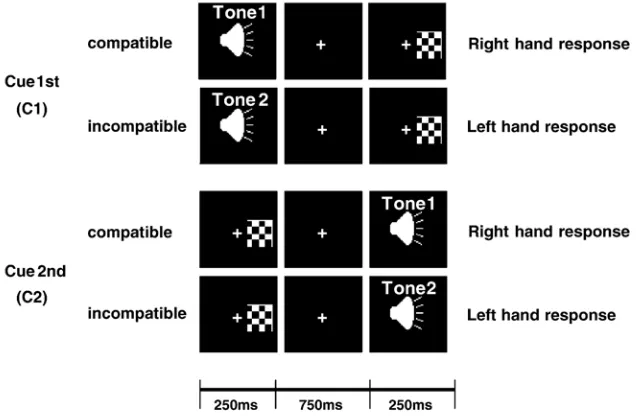
Twelve healthy adult subjects aged 18–33 (8 males) were presented with two stimuli: a high or low pitch binaural tone and a checkerboard square presented left or right of fixation (Fig. 1). Each stimulus was presented for 250 ms. The auditory stimulus represented a cue, while the visual stimulus represented a target. In one block of trials, the C1 task, the cue was presented first and was followed by the target. In another block of trials, the C2 task, the cue was presented second and was preceded by the target. The inter-stimulus interval was 1000 ms. After the second stimulus subjects responded by button press. The tone’s pitch indicated whether a response was required to be spatially compatible or incompatible, i.e., with the hand on the same or opposite side of the target. High pitch (250 Hz) and low pitch (4000 Hz) tones were used to indicate compatible and incompatible responses, respectively. The pitch was randomly varied across trials. Subjects were given 1050 ms to respond after the second stimulus. This was followed by an inter-trial interval that varied between 800 and 1200 ms.
Control tasks were run where the tone had no meaning and the response rule was fixed as either compatible or incompatible within a block of trials. These were denoted C1c and C2c, depending on whether the auditory stimulus was presented first or second. Each
of the four tasks (C1, C2, C1c, C2c) contained four conditions determined by the side of the target and compatibility of the response (LC = left compatible, LI = left incompatible, RC = right compatible, RI = right incompatible), bringing the total number of conditions to 16.
EEG recordings and preprocessing
Continuous electroencephalogram (EEG) recordings were digitized using NeuroScan 4.0 with a 65 channel ElectroCap at a 250 Hz sampling rate. Electrodes were referenced to Cz during the recording. In addition, electro-oculogram (EOG) recordings were made and subsequently used for PCA based correction of ocular artifacts in continuous EEG data (Picton et al., 2000). The continuous data were re-referenced to an average reference and bandpass filtered (0.5–45 Hz). Data were epoched into 2200 ms epochs (550 time points at 250 Hz sampling rate) time-locked to the onset of the first stimulus and 200 ms prestimulus baseline. The epoch length was sufficient to include both stimuli and the response. Epoched data sets containing trials with correct responses were further cleaned of artifacts using independent component analysis (ICA) as implemented in EEGLAB software (Delorme and Makeig, 2004) and run in MATLAB (Mathworks Inc.). Since most of the ocular artifacts were previously corrected, ICA based artifact removal and correction consisted of the following steps: (1) trials contaminated with excessive amplitudes were removed first, (2) an ICA decomposition was performed on the remaining concatenated trials and (3) components carrying residual ocular and muscle artifacts were subtracted. Each subject’s data set was divided into 16 condition-specific sets of trials. The number of artifact-free, correct-response trials per subject, per condition was between 20 and 56, with average 45.
Data organization for group ICA
Data from all subjects and conditions were combined into a single matrix in order to: (1) incorporate data from all subjects and conditions, (2) equalize number of trials across subjects and
conditions, (3) increase signal-to-noise ratio while preserving temporal dynamics and (4) reduce the computational load for subsequent ICA decomposition. We utilized the following sorting and subaveraging procedure. Subject and condition-specific trials were sorted with respect to the response time (RT), from faster to slower. Sorted trials were binned into 5 bins with approximately the same number of trials per bin (9 on average). Data were averaged within each bin, resulting in a set of 5 subaveraged trials per subject and condition. RT was calculated as an offset in ms from the second stimulus onset. The average RT and average standard deviation of RT across subjects and conditions were 460 ms and 114 ms, respectively. Thus, the activation of motor response typically ranged by at least 200 ms. Subaveraging across trials with vastly different response times would introduce temporal smearing and obscure response locked activations. We first ordered the trials with respect to RT so that the subsequent binning and subaveraging would preserve the overall temporal characteristics of single trials in terms of both stimulus and response locked activation patterns. In view of the constraints presented by the number of available trials, RT variability and the computational load, the number of bins was experimentally determined as most appropriate.
The subaveraged trials were concatenated into a single data set representative of all conditions and subjects. The resulting data matrixXwas 65 ×min size, where 65 = number of electrodes and m= number of conditions * number of subjects * number of sub-averaged trials * number of time points per trial = 16 * 12 * 5 * 550 = 528,000.
Group ICA
Spatial dimensionality reduction via PCA followed by Infomax ICA decomposition was performed on the group data matrixX, described above. X was initially decomposed with PCA and spatially reduced to a subspace spanned by a proposed number of components. The basis of the subspace was then rotated using the Infomax algorithm as implemented in EEGLAB. The effect of the initial PCA procedure was to determine a subspace that captured a portion of the variance across electrodes and was spanned by an orthogonal basis. The purpose of the subsequent Infomax procedure was to find another basis for the same subspace such that spanning components were no longer necessarily orthogonal, but rather maximally temporally independent in the Infomax sense, i.e., with maximum component joint entropy. For a given model with p components, the PCA followed by ICA decomposition resulted in a p× 65 weighting matrix, which expressed each component as a weighted sum of electrodes (see Appendix A for details). A single trial time series of the derived components were obtained by multiplying the electrode single trial time series by the weighting matrix.
ðcomponent activationsÞptime¼ ðweighting matrixÞp65
Tðelectrode activationsÞ65time
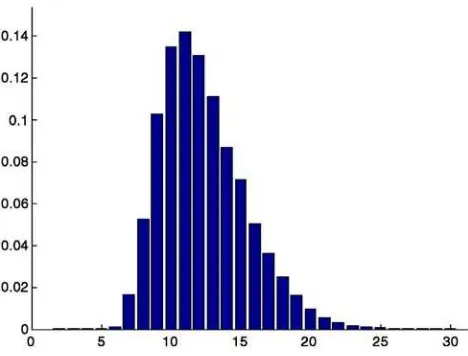
An optimal number of ICA components was determined using Bayesian Information Criterion (BIC) (Hansen et al., 2001). Models with the number of components ranging from 1 to 65 were considered, thus covering the entire theoretical range, and a Bayesian probability of each model was evaluated. The model with maximum probability was selected for subsequent PLS analysis.
PLS analysis in electrode space
A complete description of PLS can be found inLobaugh et al. (2001)andMcIntosh (2004). Here we present the essential details with a brief mathematical description in Appendix B. PLS starts with a data matrix composed such that the rows correspond to subjects within conditions and the columns correspond to time points within electrodes. Each row of the matrix consists of a condition and subject-specific average time series, horizontally concatenated across electrodes. In the grand mean deviation analysis, grand average time series for each condition are calculated and the data matrix is mean-centered column-wise with respect to condition-specific grand averages.
The mean-centered matrix is decomposed using singular value decomposition (SVD) to produce a set of mutually orthogonal latent variables (LVs, which are the left and right singular vectors from the SVD) with decreasing order of magnitude (analogously to PCA). Each LV consists of: (1) a singular value, (2) a design LV and accompanying design saliences (weights within the right singular vector) representing a task contrast and (3) scalp LV and accompanying electrode saliences (weights within the left singular vector) representing the optimal spatiotemporal relation to the identified contrast. The relative strength of each LV can be evaluated by computing the percentage of cross-block covariance accounted for. This is the ratio of the squared singular value over the summed squared singular values for all LVs. This metric is not to be confused with the percentage of total variance accounted for as it pertains only to the covariance between measured brain activity and experimental design and thus is dependent on the parameterization of the design.
The figure of merit for PLS is provided by statistical assessment using resampling procedures. Firstly, the singular value for each LV is tested for significance based on permutation tests, which randomly reassign conditions within subjects. Secondly, the electrode saliences of the significant LVs are further tested for stability across subjects, by bootstrap resampling of subjects within conditions. The ratio of the salience to the bootstrap standard error is approximately equivalent to az-score and is used as a measure of stability. Thresholding bootstrap ratios allow identification of electrodes and time points (spatiotemporal pattern) of stable LV expressions. In summary, grand mean deviation PLS analysis identifies main data driven task effects (e.g., as inFig. 2) together with their respective spatiotemporal signatures, which are stable across subjects.
In the non-rotated (hypothesis driven) version of PLS analysis, a set of a priori contrasts is constructed and the sums-of-squares for the projection of each contrast on the data are computed (McIntosh, 2004). Once again, statistical assessment assigns ap-value to the sums-of-squares for each contrast projection and identifies corresponding stable spatiotemporal patterns.
PLS analysis in component space
representation of the data also implied a new interpretation of the task contrasts in terms of the spatiotemporal patterns. Both mean-centering and non-rotated versions of PLS were used in the analysis of the component data.
Comparison of PLS results in electrode and component spaces
In the first set of PLS analyses we used a mean-centering approach in order to identify the main effects due to condition differences (LC, LI, RC, RI) within four main tasks (C1, C2, C1c and C2c). We used a randomization scheme with 500 permutations for contrast significance estimation and 500 bootstrap samples for the estimation of the stability of spatiotemporal contrast saliences. We compared task contrasts of the first three latent variables in electrode and component analyses, along with their corresponding
p-values calculated by the permutation tests and cross-block covariance contributions.
In the second set of analyses we used a non-rotated version of PLS in order to assess statistical properties of three a priori contrasts. With a condition ordering LC, LI, RC and RI, the contrasts were: visual field (1, 1,−1,−1), compatibility (1,−1, 1,
−1) and hand of response (1,−1,−1, 1). LC and RI both require a
left-hand response, while LI and RC require a right-hand response. As with the mean-centered analysis, the non-rotated PLS analysis was done within the four main tasks. This gave us an opportunity to make a direct comparison between four sets of electrode and component analyses using identical contrasts. For each of the three contrasts, we compared significance and percent cross-block covariance.
Comparison of PLS results between original electrode data, filtered electrode data and component data
To foreshadow, we found overall enhancement of task effects in the component space compared to the electrode space, as a result of data reduction and filtering (see Results). In order to investigate the effect of group ICA filtering directly, we back-projected the component signal into the electrode space (see Appendix A for
details). We performed mean-centering PLS analyses on the filtered electrode data and compared the results with those from the PLS analyses on the original, unfiltered electrode data. We then calculated the dot products between the design LV vectors from filtered and unfiltered data analysis to assess their similarity. Because the vectors are unit length, the dot products are cosines or correlations.
Direct comparison between spatiotemporal patterns of task related differences was investigated using the three contrasts. For this purpose, we calculated the dot product between saliences in the original and filtered electrode spaces both of which were scaled to unit length.
Finally, we performed a three-way comparison between original electrode data, filtered electrode data and component data. We used a mean-centering PLS approach in order to identify the main effects within task pairs (C1 and C1c, C2 and C2c, C1 and C2, C1c and C2c). Each task pair consisted of 8 conditions. This allowed more extensive statistical assessment over increased number of conditions with potential for larger number of orthogonal contrasts. We compared electrode and component PLS results in terms of the number of significant LVs and corresponding percent cross-block covariances. Because mean-centered PLS produces orthogonal contrasts, we summed up the total cross-block covariance across significant LVs. This was taken as a measure of the portion of the cross-block covariance captured by the significant contrasts. We also calculated the relative weight of stable spatiotemporal patterns in the following way. For each significant LV, we calculated the number of space–time points that stably expressed the design contrast across subjects (absolute bootstrap ratio > 3.3). The number was then represented as a percent of the total number of space–time points to adjust for the differing number of spatial coordinates in electrode and components spaces. This measure was taken as an estimate of the efficiency for a given data representation: larger percent of space–time with stable contrast expression indicated more efficient representation.
Results
Group ICA components
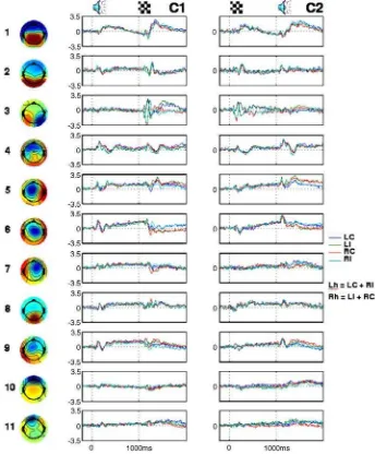
The maximum BIC probability was obtained for the model with 11 group ICA components, as shown inFig. 2. The data set was accordingly reduced and decomposed into 11 maximally temporally independent modes whose topographic scalp maps together with grand average time series in all conditions from C1 and C2 tasks are shown in Fig. 3. Two last components were identified as artifactual based on their scalp maps and time courses across subjects and subaveraged trials, using similar criteria as in single subject artifact rejection (Delorme and Makeig, 2004). Unlike task related components, artifactual components lack consistent time-locked and task related amplitude variations, as illustrated inFig. 4. The last two components were dropped from further analysis.
The nine task related components exhibit a great deal of temporal specificity pointing to separate functional roles. For example, components 2 and 3 are mostly involved in visual response because their highest activation amplitudes are occurring 50–300 ms after the onset of the visual stimulus and are otherwise at the baseline level. In particular, component 3 shows strong differentiation between left and right visual field, which extends for at least 800 ms following the onset of the visual stimulus. Fig. 2. Probability distribution across models varying in number of group
Components 4 and 6 activate strongly 50–300 ms after the onset of the auditory stimulus. Motor response is mostly carried by components 5, 6 and 9, with strong differentiation for left hand (LC and RI) and right hand (LI and RC) response. Component 8 shows weak task related activation and further investigation of its single trial time series and power spectrum indicated that this component captured alpha rhythms with sporadic stimulus locking (data not shown), consistent with its topographic map indicative of the visual cortex.
PLS results in electrode and component spaces
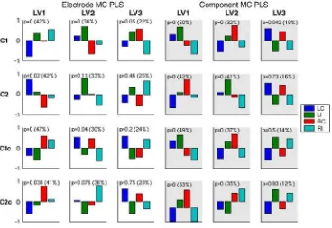
Results from mean-centering PLS analyses across four main tasks in electrode and component spaces are shown inFig. 5. For both analyses, the obtained sets of design LVs are overall expressing three contrasts: left visual field vs. right visual field
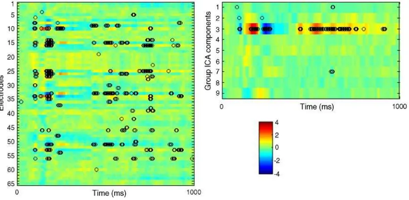
(Lvf vs. Rvf), high vs. low tone frequency, i.e., compatible vs. incompatible (C vs. I), and left vs. right hand response (Lh vs. Rh). Table 1shows the comparison of the non-rotated PLS analysis in terms of significance and percent cross-block covariance. The comparison of the spatiotemporal patterns characterizing the three contrasts is more complicated because of the different spatial representations. In general, the electrode space exhibited patterns with more overlap in both space and time. This is illustrated inFig. 6. It shows spatiotemporal patterns for the Lvf vs. Rvf contrast in the C2 task. In both spaces the signal differentiation for left and right visual field expresses strongly during 150–250 ms after stimulus onset and then re-emerges during the slow wave period (400–800 ms) when subjects memorize the side of the visual field while waiting for the cue. While this differentiation extends over several electrodes in the electrode space, it is compactly captured by a single group ICA component, namely component 3. Fig. 3. Scalp maps of the eleven group ICA components and their grand average time series across four conditions in C1 and C2 tasks. Scalp maps were produced using spherical spline interpolation. In time series plots,Y-axis represents component activation amplitude inμV andX-axis represents time. 0 and 1000 ms
PLS results in original electrode data, filtered electrode data and component data
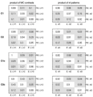
Results from the comparison between original and filtered electrode data via dot products of design LVs from mean-centering PLS are shown in the left column of Fig. 7. Products on the diagonal are close to 1, and off the diagonal are close to 0. This indicates that the sets of contrasts were not only similar across all
four tasks, but their ordering by the contribution to the cross-block covariance was also the same. Though the contrast sets were highly similar, they were not identical.
To investigate spatiotemporal patterns for identical experimen-tal effects we subsequently performed non-rotated PLS analyses with the three a priori contrasts and then compared the associated spatiotemporal patterns of the original and filtered electrode analyses. The resulting dot products of the normalized salience
Fig. 5. Mean-centering PLS analysis of electrode data (left) and component data (right) across the four main tasks. Shown are three design LVs from each analysis, along with their correspondingp-values and percent cross-block covariance. Design LVs express contrasts between 4 conditions, LC, LI, RC and RI. Fig. 4. Component activations across sorted group data are visualized using ERP image tool of EEGLAB. Trials are stacked vertically with task order C1, C2, C1c and C2c from bottom to top, and within each task in condition order LC, LI, RC and RI from bottom to top. Trial time interval (from−200 to 2000 ms)
corresponds to the horizontal axis and color represents activation amplitude inμV. Visual stimulus onset is at 1000 ms in C1 and C1c tasks and at 0 ms in C2 and
vectors are shown in Fig. 7 on the right. Once again, the dot product matrices resemble the 3 × 3 identity matrix, which indicates high degree of similarity between the two sets of spatiotemporal patterns of the a priori contrasts.
Results from the three-way comparison between PLS analyses of the original electrode data, filtered electrode data and component data are summarized in Table 2. Mean-centering PLS analyses were performed on paired tasks. For each task pair and data type, shown is the number of significant LVs, the corresponding cross-block covariance contributions and percent of space–time with stable contrast expression. In general, analysis of component data produced the largest number of significant effects and stable time points, whereas the original electrode data produced the fewest. This was most evident on the analysis of C2 vs. C2c, where the analysis of component data yielded 3 significant LVs, while the original data yielded only one. The filtered data produced an intermediate result, with 2 significant LVs.
Discussion
In the standard ERP analysis, the spatiotemporal representation of data uses time series of the electrode recordings averaged across
repeated trials for each subject. Spatial smearing and signal redundancy of the recorded signal are also reflected in analysis results. This can make identification and spatiotemporal separation of task effects difficult. In this paper, we introduced an alternative approach to ERP signal representation. We utilized group PCA data reduction and group ICA filtering in order to re-express the signal in a compressed and efficient way, with optimum balance between goodness of fit and model complexity as determined by Bayesian Information Criterion. In an application to real EEG we were able to compress the spatial representation of the data to a small set of maximally temporally independent scalp topographies (group ICA components), with relatively specialized functional relevance.
Similar spatiotemporal PCA and ICA based techniques have been previously used for data reduction and filtering (Spencer et al., 1999; Curran and Friedmann, 2004; Makeig et al., 1999). In these studies the analyses were performed on either grand averaged electrode time series (Makeig et al., 1999) or on combined subject averages (Spencer et al., 1999; Curran and Friedmann, 2004). Both averaging procedures may impact temporal specificity, especially in experiments with large variability in brain response latency. This is commonly observed in experiments requiring behavioral responses such as a button press. In order to increase the
signal-Fig. 6. Spatiotemporal patterns in electrode and component spaces characterizing Lvf vs. Rvf contrast in C2 task where visual stimulus onset starts at 0 ms. Each colored horizontal line represents electrode or component salience across time. Hot colors signify space–time points with positive contrast expression, i.e., where signal is higher for left than for right visual filed. Analogously, cool colors signify points with negative contrast expression, i.e., where signal is higher for right than for left visual field. Black circles identify space–time points for which contrast expression is stable across subjects (absolute bootstrap ratio > 3.3). Table 1
p-values for the three ideal contrasts in electrode (E) and component (C) analyses
C1 C2 C1c C2c
p Cc (%) p Cc (%) p Cc (%) p Cc (%)
E Lvf vs. Rvf 0 37 0.03 39 0 46 0.04 39
C vs. I 0 40 0.4 0.03 30 0.7
Lh vs. Rh 0.04 24 0.08 0.2 0.7
C Lvf vs. Rvf 0 47 0 41 0 48 0 36
C vs. I 0.04 19 0.7 0.4 0.7
Lh vs. Rh 0 34 0 42 0 37 0 51
to-noise ratio and at the same time preserve temporal specificity, we chose the middle ground between single trial data and subject averages. This was done by a subaveraging procedure, which divided each subject’s trials into several temporally consistent bins and then calculated the average time series for each bin. The data matrix combining the subaverages from bins across all subjects and conditions was analyzed and compressed using PCA and ICA. The
resulting set of ICA components was representative of the group across all experimental conditions.
Under the spatial compression from full electrode space onto group ICA space, task effects were not only preserved, but also further enhanced in terms of statistical properties. This was demonstrated by an increased number of significant task effects in the group ICA space, compared to both original and filtered
Table 2
Comparison of significant task effects in mean-centering PLS analyses of original electrode (E), filtered electrode (FE) and component (C) data across combined tasks
C1, C1c C2, C2c C1, C2 C1c, C2c
E sig LVs 3 1 2 2
cc (%) 39 21 14 (74) 65 (65) 63 9 (72) 60 12 (72)
st (%) 12 5 5 (22) 13 (13) 18 8 (26) 11 4 (15)
FE sig LVs 3 2 2 2
cc (%) 39 22 14 (75) 64 11 (75) 64 9 (73) 63 11 (74)
st (%) 14 5 5 (24) 14 3 (17) 20 9 (29) 14 5 (19)
C sig LVs 4 3 4 4
cc (%) 38 27 13 9 (87) 32 25 23 (80) 38 21 14 12 (85) 35 25 16 11 (87) st (%) 8 8 4 4 (24) 8 8 4 (20) 10 11 6 3 (30) 8 14 4 3 (29)
For each analysis, sig LVs denotes number of significant LVs (p< 0.05), cc denotes percent cross-block covariance for significant LVs with sum over all significant LVs given in parentheses and st denotes percent of space–time that stably expresses significant LVs (absolute bootstrap ratio > 3.3) with sum over all significant LVs given in parentheses.
electrode spaces (Table 2). Note that there was no attempt to preserve maximum variance by the compression. For example, the subspace spanned by initial 11 PCA/ICA components captured 93% variance of the data matrix variance. After rejecting 2 artifact-related components, the space spanned by the remaining 9 ICA components captured only 82% of the variance. However, task effects exhibited by the 9 group ICA components were enhanced. Although filtered electrode data showed some enhancement of task effects compared to the original electrode data (greater or equal number of significant contrasts with larger contributions to cross-block covariance and enhanced stability of spatiotemporal patterns), it was not nearly as good as in the component data. Despite filtering with ICA, it is likely that the residual noise from less heavily weighted electrodes continues to attenuate task effects.
Overall, group ICA component space offers efficient spatial representation with increased sensitivity to task related signal differences and can therefore be used as an alternative or as a complement to the more traditional electrode space.
Acknowledgments
This work was supported by CIHR and J.S. McDonnell foundation. We thank Stephen Strother for helpful suggestions and discussions. We also thank Mackenzie Glaholt, Maya Stefanovic and Andrea Diaconescu for data acquisition and preprocessing. All code used for Group ICA and for PLS analysis can be accessed through www.rotman-baycrest.on.ca/pls or by contacting the authors. The Group ICA module will also be made available as a plug-in for EEGLAB.
Appendix A
We present a description of the data transformation using PCA dimensionality reduction followed by ICA rotation and further reduction. LetXbe a data matrix containing time series concatenated across subaveraged trials, as described in the Materials and methods section. The size ofX is 65 ×m, where 65 = number of electrodes and m= number of time points from the concatenated subaveraged trials. The matrix Wof eigenvec-tors of the matrix of observed covariances C=XXT, is defined by:
XXT¼WEWT;
where Wis orthogonal andE is diagonal and both matrices are 65 × 65 in size. Projection ofX onto a subspace defined by the first p principal components is obtained as:
Y¼WpTX;
whereWpis a 65 ×pmatrix containing the firstpcolumns ofW. Yis subsequently rotated with ICA into a new coordinate space of temporally independent components
Z¼ RY;
whereRis an invertiblep×pmatrix. Lettingp range between 1 and 65, the corresponding ICA spaces are evaluated using Bayesian Information Criterion and optimalpis selected (for our data set, the optimal p was 11). Subsequent ICA filtering of residual artifacts is achieved by restrictingZto the subspace Zq
spanned by the first q components (after possibly resorting the rows ofR so that unwanted components are last):
Zq¼RqY;
where Rqdenotes matrix containing the first q rows ofR. ICA filtered version ofYsignal is obtained by back-projecting theZq space
YF¼ ðR 1ÞqZq¼ ðR 1ÞqRqY;
where (R−1)
q denotes a p×q matrix containing the first q columns ofR−1. It is easy to check thatR
q(R−1)q=Iq, whereIq denotes the identity matrix of size q×q.
Finally, PCA and ICA filtered version of the original electrode signal is obtained by back-projecting the YF signal into the electrode space
XF¼WpYF¼WpðR 1ÞqRqY¼WpðR 1ÞqRqWpTX:
In summary: (1) the relationship between the original electrode signal and retained ICA component signal is given byZq=L X, whereL=RqWpTis aq× 65 weighting matrix and (2) PCA–ICA filtered electrode signal is given byXF=P X, whereP=Wp(R−1)q RqWpTis a 65 × 65 filtering matrix. It can be easily shown thatWp (R−1)qis the Moore
–Penrose pseudoinverse ofL.
This filtering process can now be applied to every set of subject and condition-specific single trial data. Ifxdenotes a data matrix of size 65 ×ncontaining the original electrode single trial time series withntime points, then the matrix of single trial activations for the group ICA components is given byzq=L x, and filtered single trial electrode time series is given byxF=P x.
Appendix B
B.1.Grand mean deviation PLS analysis
Assume a rectangular matrixMwithnobservations (subjects) andkconditions as then*krows. The columns of the data matrix contain the signal measured for each electrode or independent component at each time point. The first column has intensity for the first electrode/component at the first time point, the second column has the intensity at the second time point. With m electrodes/components andttime points, there arem*tcolumns in the matrixM. Column-wise averages are created within each task, yielding matrixT, akbym*tmatrix of task means. Grand mean deviation matrixTdevis defined as
Tdev¼T 1Tð1TTTÞ=k; ð1Þ
where matrix 1 is a column vector of ones of length k and T denotes a matrix transpose.Tdevis a column-wise mean-centered matrix (for this reason, this version of PLS is also called the “mean-centered”task PLS). The operation:
½ScalpLV;S;DesignLV ¼SVDðTdevTÞwhere : ð2Þ
ScalpLVTSTDesignLVT¼TdevT ð3Þ
representing the grand mean, which is eliminated through mean-centering.
B.2. Non-rotated PLS
We start with a set of contrastsCcomparing specific tasks (e.g., Helmert contrasts, dummy coded contrasts). Next the contrasts are projected on to matrixT:
CTTT¼E: ð4Þ
The sums-of-squares for each vector in E are computed and treated to the same permutation assessment as the singular values derived in Eq. (2). The weights within each vector of Eare the electrode/component saliences, whose reliability is assessed with bootstrap resampling. While the non-rotated PLS has the advantage of allowing a direct assessment of hypothesized experimental effects, the interpretation may be difficult if non-orthogonal contrasts are used.
References
Addis, D.R., McIntosh, A.R., Moscovitch, M., Crawley, A.P., McAndrews, M.P., 2004. Characterizing spatial and temporal features of autobio-graphical memory retrieval networks: a partial least squares approach. NeuroImage 23, 1460–1471.
Curran, T., Friedmann, W.J., 2004. ERP old/new effects at different retention intervals in recency discrimination tasks. Cogn. Brain Res. 18 (2), 107–120.
Delorme, A., Makeig, S., 2004. EEGLAB: an open source toolbox for analysis of single-trial EEG dynamics. J. Neurosci. Methods 134, 9–21.
Duzel, E., Habib, R., Schott, B., Schoenfield, A., Lobaugh, N.J., McIntosh, A.R., Scholz, M., Heinze, H.J., 2003. A multivariate, spatiotemporal
analysis of electromagnetic time–frequency data of recognition memory. NeuroImage 18, 185–197.
Friston, K.J., Holmes, A.P., Price, C.J., Buchel, C., Worsley, K.J., 1999. Multisubject fMRI studies and conjunction analyses. NeuroImage 10, 385–396.
Hansen, K., Larsen, J., Kolenda, T., 2001. Blind detection of independent dynamic components. IEEE Int. Conf. Acoust. Speech Signal Process. 5, 3197–3200.
Hay, J.F., Kane, K.A., West, R., Alain, C., 2002. Event-related neural activity associated with habit and recollection. Neuropsychologia 40, 260–270.
Itier, R.J., Taylor, M.J., 2002. Inversion and contrast polarity reversal affect both encoding and recognition process of unfamiliar faces: a repetition study using ERP’s. NeuroImage 15, 353–372.
Lobaugh, N.J., West, R., McIntosh, A.R., 2001. Spatiotemporal analysis of experimental differences in event-related potential data with partial least squares. Psychophysiology 38, 517–530.
Makeig, S., Westerfield, M., Townsend, J., Jung, T.-P., Courchesne, E., Sejnowski, T.J., 1999. Functionally independent components of early event-related potentials in a visual spatial attention task. Philos. Trans. R. Soc. Lond., B Biol. Sci. 354, 1135–1144.
Makeig, S., Delorme, A., Westerfield, M., Jung, T.-P., Townsend, J., Courchesne, E., Sejnowski, T.J., 2004. Electroencephalographic brain dynamics following manually responded visual targets. PLoS Biol. 2, e176. McIntosh, A.R., 2004. Partial least squares analysis of neuroimaging data:
applications and advances. NeuroImage 23 (Suppl. 1), S250–S263. Picton, T.W., Van Roon, P., Armilio, M.L., et al., 2000. The correction of
ocular artifacts: a topographic perspective. Clin. Neurophysiol. 111 (1), 53–65.
Spencer, K.M., Dien, J., Donchin, E., 1999. A componential analysis of the ERP elicited by novel events using a dense electrode array. Psychophysiology 36, 409–414.