Leverage and Capital Structure week 10 and 11

(1)

Chapter 12

Leverage

(2)

Learning Goals

1. Discuss leverage, capital structure, breakeven

analysis, the operating breakeven point, and the effect of changing costs on it.

2. Understand operating, financial, and total leverage and the relationship among them.

3. Describe the basic types of capital, external

(3)

(4)

Learning Goals

4. Explain the optimal capital structure using a graphical view of the firm’s cost of capital functions and a zero-growth valuation model.

5. Discuss the EBIT-EPS approach to capital structure. 6. Review the return and risk of alternative capital

(5)

Leverage

• _Leverage_{results from the use of fixed-cost assets or funds to}

magnify returns to the firm’s owners.

• _{Generally, increases in leverage result in increases in}_{risk and}

return, whereas decreases in leverage result in decreases in risk and return.

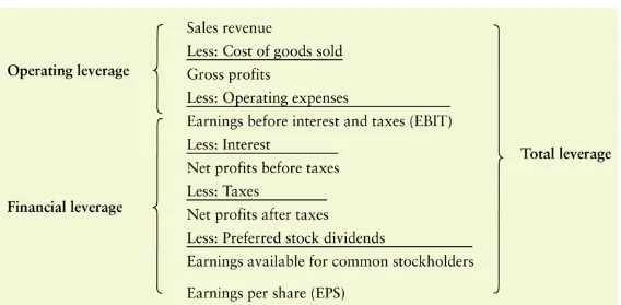
• _{The amount of leverage in the firm’s}_{capital structure}_{—the mix}

(6)

Leverage (cont.)

(7)

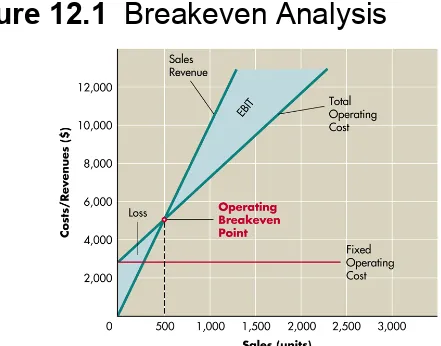
Breakeven Analysis

• _{Breakeven (cost-volume-profit) analysis}_{is used to:}

– _{determine the level of operations necessary to cover all}

operating costs, and

– _{evaluate the profitability associated with various levels of}

sales.

• _{The firm’s}_{operating breakeven point (OBP)}_{is the}

level of sales necessary to cover all operating expenses.

(8)

Breakeven Analysis (cont.)

• _{To calculate the OBP, cost of goods sold and operating expenses}

must be categorized as fixed or variable.

• _{Variable costs vary directly with the level of sales and are a}

function of volume, not time.

• _{Examples would include direct labor and shipping.}

• _{Fixed costs are a function of time and do not vary with sales}

volume.

(9)

P = sales price per unit Q = sales quantity in units

FC = fixed operating costs per period VC = variable operating costs per unit

EBIT = (P x Q) - FC - (VC x Q)

Breakeven Analysis:

Algebraic Approach

• _{Letting EBIT = 0 and solving for Q, we get:}

Using the following variables, the operating portion of a firm’s income statement may be recast as

(10)

Breakeven Analysis:

(11)

Breakeven Analysis:

Algebraic Approach (cont.)

(12)

Q = $2,500 = 500 posters $10 - $5

Breakeven Analysis:

Algebraic Approach (cont.)

• _{This implies that if Cheryl’s sells exactly 500}

Example: Cheryl’s Posters has fixed operating

costs of $2,500, a sales price of $10 per

(13)

EBIT = (P x Q) - FC - (VC x Q)

EBIT = ($10 x 500) - $2,500 - ($5 x 500)

EBIT = $5,000 - $2,500 - $2,500 = $0

Breakeven Analysis:

Algebraic Approach (cont.)

• We can check to verify that this is the case by

(14)

Breakeven Analysis:

Graphical Approach

(15)

Assume that Cheryl’s Posters wishes to evaluate the impact of several options: (1) increasing fixed operating costs to

$3,000, (2) increasing the sale price per unit to $12.50, (3) increasing the variable operating cost per unit to $7.50, and (4) simultaneously implementing all three of these changes.

(16)

(1) Operating BE point = $3,000/($10-$5) = 600 units

(2) Operating BE point = $2,500/($12.50-$5) = 333 units

(3) Operating BE point = $2,500/($10-$7.50) = 1,000 units

(4) Operating BE point = $3,000/($12.50-$7.50) = 600 units

(17)

Breakeven Analysis: Changing Costs

and the Operating Breakeven Point

(18)

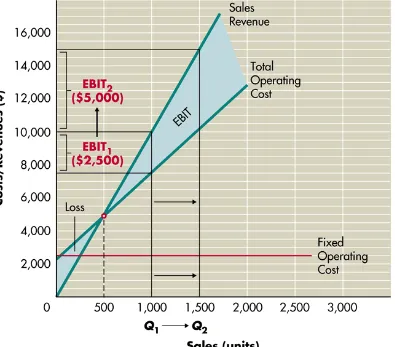
Operating Leverage

Figure 12.2

(19)

Operating Leverage (cont.)

(20)

Operating Leverage: Measuring the

Degree of Operating Leverage

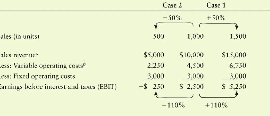
• _The_{degree of operating leverage (DOL)}_{measures the}

sensitivity of changes in EBIT to changes in Sales.

• _{A company’s DOL can be calculated in two different}

ways: One calculation will give you a point estimate, the other will yield an interval estimate of DOL.

• _{Only companies that use fixed costs}

(21)

DOL = Percentage change in EBIT Percentage change in Sales

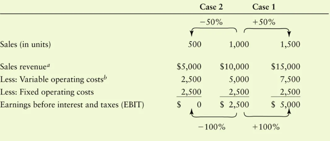
Case 1: DOL = (+100% ÷ +50%) = 2.0

Case 2: DOL = (-100% ÷ -50%) = 2.0

Operating Leverage: Measuring the

Degree of Operating Leverage (cont)

• _{Applying this equation to cases 1 and 2 in Table}

(22)

DOL at base Sales level Q = Q X (P – VC) Q X (P – VC) – FC

Substituting Q = 1,000, P = $10, VC = $5, and FC = $2,500 yields the following result:

Operating Leverage: Measuring the

Degree of Operating Leverage (cont)

• A more direct formula for calculating DOL at a base

(23)

Assume that Cheryl’s Posters exchanges a portion of its variable operating costs for fixed operating costs by

eliminating sales commissions and increasing sales

salaries. This exchange results in a reduction in variable costs per unit from $5.00 to $4.50 and an increase in

fixed operating costs from $2,500 to $3,000

DOL at 1,000 units = 1,000 X ($10 - $4.50) = 2.2 1,000 X ($10 - $4.50) - $2,500

(24)

Operating Leverage: Fixed Costs

and Operating Leverage (cont.)

(25)

Financial Leverage

• Financial leverage results from the presence of fixed

financial costs in the firm’s income stream.

• _{Financial leverage can therefore be defined as the}

potential use of fixed financial costs to magnify the effects of changes in EBIT on the firm’s EPS.

• The two fixed financial costs most commonly found on

(26)

Chen Foods, a small Oriental food company, expects EBIT of $10,000 in the current year. It has a $20,000 bond with a

10% annual coupon rate and an issue of 600 shares of $4 annual dividend preferred stock. It also has 1,000 share of common stock outstanding.

(27)

Financial Leverage (cont.)

(28)

Financial Leverage: Measuring the

Degree of Financial Leverage

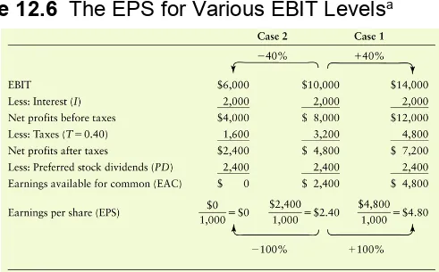
• _The_{degree of financial leverage (DFL)}_{measures the}

sensitivity of changes in EPS to changes in EBIT.

• _{Like the DOL, DFL can be calculated in two different}

ways: One calculation will give you a point estimate, the other will yield an interval estimate of DFL.

• _{Only companies that use debt or other forms of fixed}

(29)

DFL = Percentage change in EPS Percentage change in EBIT

Case 1: DFL = (+100% ÷ +40%) = 2.5

Case 2: DFL = (-100% ÷ -40%) = 2.5

• _{Applying this equation to cases 1 and 2 in Table}

12.6 yields:

(30)

DFL at base level EBIT = EBIT

EBIT – I – [PD x 1/(1-T)]

Substituting EBIT = $10,000, I = $2,000, PD = $2,400, and the tax rate, T = 40% yields the following result:

DFL at $10,000 EBIT = $10,000

• A more direct formula for calculating DFL at a base

level of EBIT is shown below.

(31)

Total Leverage

• Total leverage

results from the combined effect

of using fixed costs, both operating and

financial, to magnify the effect of changes in

sales on the firm’s earnings per share.

• Total leverage can therefore be viewed as the

(32)

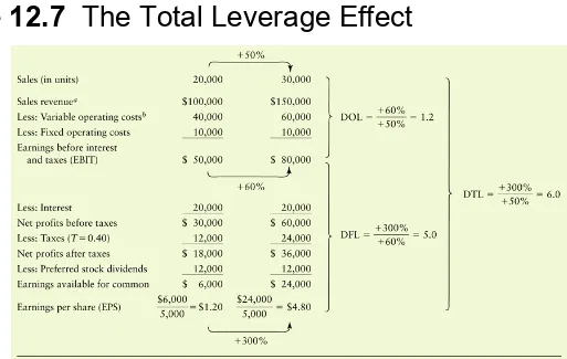
Cables Inc., a computer cable manufacturer, expects sales of 20,000 units at $5 per unit in the coming year and must meet the following obligations: variable operating costs of $2 per unit, fixed operating costs of $10,000, interest of $20,000, and preferred stock dividends of $12,000. The firm is in the 40% tax bracket and has 5,000 shares of common stock

(33)

DTL = Percentage change in EPS Percentage change in Sales

Degree of Total Leverage (DTL) = (300% ÷ 50%) = 6.0

Total Leverage: Measuring the

Degree of Total Leverage

• _{Applying this equation to the data Table 12.7}

(34)

DTL at base sales level = Q x (P – VC)

• A more direct formula for calculating DTL at a base

level of Sales, Q, is shown below.

(35)

DTL = DOL x DFL

The relationship between the DTL, DOL, and DFL is illustrated in the following equation:

DTL = 1.2 X 5.0 = 6.0 Applying this to our previous example we get:

(36)

Total Leverage (cont.)

(37)

The Firm’s Capital Structure

• Capital structure is one of the most complex areas of

financial decision making due to its interrelationship with other financial decision variables.

• _{Poor capital structure decisions can result in a high cost}

of capital, thereby lowering project NPVs and making them more unacceptable.

• _{Effective decisions can lower the cost of capital,}

(38)

(39)

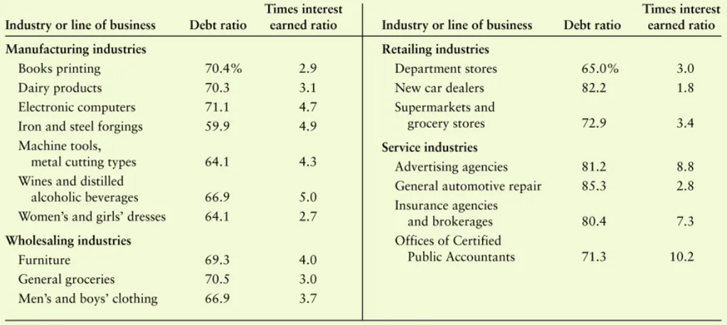
External Assessment of Capital Structure

(40)

Capital Structure of Non-U.S. Firms

• In recent years, researchers have focused attention not

only on the capital structures of U.S. firms, but on the capital structures of foreign firms as well.

• _{In general, non-U.S. companies have}_{much higher}

degrees of indebtedness than their U.S. counterparts.

• _{In most European and Pacific Rim countries, large}

commercial banks are more actively involved in the

(41)

Capital Structure

of Non-U.S. Firms (cont.)

• _{Furthermore, banks in these countries are permitted to make}

large equity investments in non-financial corporations—a practice forbidden in the U.S.

• _{However, similarities also exist between U.S. firms and their}

foreign counterparts.

• _{For example, the same industry patterns of capital structure tend}

to be found around the world.

• _{In addition, the capital structures of U.S.-based MNCs tend to be}

(42)

Capital Structure Theory

• According to finance theory, firms possess a target

capital structure that will minimize its cost of capital.

• _{Unfortunately, theory can not yet provide financial}

mangers with a specific methodology to help them determine what their firm’s optimal capital structure might be.

• _{Theoretically, however, a firm’s optimal capital}

(43)

• The major benefit of debt financing is the tax shield

provided by the federal government regarding interest payments.

• _{The costs of debt financing result from:}

– _{the increased probability of bankruptcy caused by debt}

obligations,

– _{the agency costs resulting from lenders monitoring the firm’s}

actions, and

– _{the costs associated with the firm’s managers having more}

information about the firm’s prospects than do investors (asymmetric information).

(44)

Capital Structure Theory:

Tax Benefits

• _{Allowing companies to}_{deduct interest}_{payments when}

computing taxable income lowers the amount of corporate taxes.

• _{This in turn increases firm cash flows and makes more}

cash available to investors.

• _{In essence, the}_{government is subsidizing}_{the cost of}

(45)

Capital Structure Theory:

Probability of Bankruptcy

• The probability that debt obligations will lead to

bankruptcy depends on the level of a company’s

business risk and financial risk.

• _{Business risk is the risk to the firm of being unable to}

cover operating costs.

• _{In general, the higher the firm’s fixed costs relative to}

variable costs, the greater the firm’s operating leverage and business risk.

• _{Business risk is also affected by revenue and cost}

(46)

Capital Structure Theory:

Probability of Bankruptcy (cont.)

• _{The firm’s capital structure—the mix between debt}

versus equity—directly impacts financial leverage.

• _{Financial leverage measures the extent to which a firm}

employs fixed cost financing sources such as debt and preferred stock.

• _{The greater a firm’s financial leverage, the greater will}

(47)

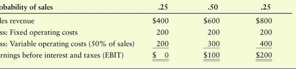
Cooke Company, a soft drink manufacturer, is preparing to make a capital structure decision. It has obtained estimates of sales and EBIT from its forecasting group as show in Table 12.9.

Capital Structure Theory:

Probability of Bankruptcy (cont.)

• _{Business Risk}

(48)

When developing the firm’s capital structure, the

financial manager must accept as given these levels of EBIT and their associated probabilities. These

EBIT data effectively reflect a certain level of business risk that captures the firm’s operating leverage, sales revenue variability, and cost predictability.

Capital Structure Theory:

Probability of Bankruptcy (cont.)

(49)

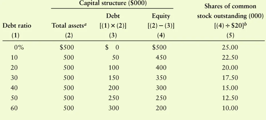
Let us assume that (1) the firm has no current liabilities, (2) its capital structure currently contains all equity, and (3) the total amount of capital remains constant at

$500,000, the mix of debt and equity associated with

Capital Structure Theory:

Probability of Bankruptcy (cont.)

(50)

Capital Structure Theory:

Probability of Bankruptcy (cont.)

• _{Financial Risk}

Table 12.10

(51)

Capital Structure Theory:

Probability of Bankruptcy (cont.)

• _{Financial Risk}

Table 12.11

Level of Debt,

(52)

Capital Structure Theory:

Probability of Bankruptcy (cont.)

(53)

Capital Structure Theory:

Probability of Bankruptcy (cont.)

(54)

Capital Structure Theory:

Probability of Bankruptcy (cont.)

(55)

Capital Structure Theory:

Probability of Bankruptcy (cont.)

(56)

Capital Structure Theory:

Probability of Bankruptcy (cont.)

• _{Financial Risk}

Figure 12.3

(57)

Capital Structure Theory:

Probability of Bankruptcy (cont.)

• _{Financial Risk}

(58)

Capital Structure Theory: Agency Costs

Imposed by Lenders

• _{When a firm borrows funds by issuing debt, the interest}

rate charged by lenders is based on the lender’s assessment of the risk of the firm’s investments.

• _{After obtaining the loan, the firm’s stockholders and/or}

managers could use the funds to invest in riskier assets.

• _{If these high risk investments pay off, the stockholders}

(59)

• _{To avoid this, lenders impose various}

monitoring costs on the firm.

• _{Examples would of these monitoring}

costs would:

– _{include raising the rate on future debt issues,} – _{denying future loan requests,}

– _{imposing restrictive bond provisions.}

(60)

Suppose management has identified an extremely lucrative investment opportunity and needs to raise capital. Based on this opportunity, management believes its stock is

Capital Structure Theory:

Asymmetric Information

• Asymmetric information results when managers of a

firm have more information about operations and future prospects than do investors.

• _{Asymmetric information can impact the firm’s capital}

(61)

In this case, management will raise the funds using debt since they believe/know the stock is undervalued

(underpriced) given this information. In this case, the use of debt is viewed as a positive signal to investors regarding the

• Asymmetric information results when managers of a

structure as follows:

Capital Structure Theory:

(62)

• Asymmetric information results when managers of a

structure as follows:

Capital Structure Theory:

Asymmetric Information (cont.)

On the other hand, if the outlook for the firm is poor,

(63)

The Optimal Capital Structure

• _{In general, it is believed that the market value of a company is}

maximized when the cost of capital (the firm’s discount rate) is minimized.

(64)

The Optimal Capital Structure

Figure 12.5

(65)

EPS-EBIT Approach

to Capital Structure

• _The_{EPS-EBIT approach}_{to capital structure involves selecting}

the capital structure that maximizes EPS over the expected range of EBIT.

• _{Using this approach, the emphasis is on maximizing the owners}

returns (EPS).

• _{A major shortcoming of this approach is the fact that earnings}

are only one of the determinants of shareholder wealth maximization.

(66)

Example

EBIT-EPS coordinates can be found by assuming specific EBIT values and calculating the EPS associated with them. Such calculations for three capital structures—debt ratios of 0%, 30%, and 60%—for Cooke Company were presented earlier in Table 12.2. For EBIT values of $100,000 and $200,000, the associated EPS values calculated are