Banking Sector Reforms and Economic Growth: Recent Evidence from a Reform-Bound Economy

P-ISSN: 2087-1228 E-ISSN: 2476-9053 Binus Business Review, 8(1), May 2017, 49-60

DOI: 10.21512/bbr.v8i1.1798

Banking Sector Reforms and Economic Growth:

Recent Evidence from a Reform-Bound Economy

Bernhard O. Ishioro

Economics Department, Faculty of the Social Sciences, Delta State University P.M.B 1, Abraka, Nigeria

ben_ishioro@yahoo.co.uk

Received: 26th _{April 2016/ Revised: 26}th _{January 2017/ Accepted: 6}th _{February 2017}

How to Cite: Ishioro, B. O. (2017). Banking Sector Reforms and Economic Growth: Recent Evidence from a Reform-Bound Economy. Binus Business Review, 8(1), 49-60.

http://dx.doi.org/10.21512/bbr.v8i1.1798

ABSTRACT

This research investigated the banking sector reforms and economic growth using time series data from 1970 to 2013 for the Nigerian economy. Autoregressive Distributed Lags (ARDL) Bounds test was applied for the specific determination of the long and short-run relationships between banking sector reforms and economic growth. The research finds that the interest rate margin is more significant than other variables in the model in explaining the banking sector reforms and economic growth. Banking sector credit to the private sector was negative and statistically insignificant in economic growth in Nigeria. This means that the size of the banking sector does not enhance economic growth. Meanwhile, inflation is negatively and statistically significant in economic growth. The duration of banking sector reforms should be defined and strictly adhered to irrespective changes in the political administration of the country.

Keywords: ARDL bounds test, banking reforms, economic growth, Nigeria

INTRODUCTION

Banking sector reforms have been regular phenomena in the Nigerian banking sector since the 1950s. According to Soludo (2007), the banking sector reforms in the early years (the 1950s) in the Nigerian financial system came in the form of legislations that were intended to strengthen the supervisory, regulatory and operational framework of the sector. The designing and implementation of the Banking Ordinance in 1952 were the first attempt aimed at reforming the sector. The ordinance was enacted to forestall the banking sector distress emanating from the unregulated establishment of banks and the consequent collapse of 22 of the 25 indigenous banks established between 1927 and 1957.

The Central Bank of Nigeria (CBN) Act of 1958 was the second among the earlier banking sector reforms. Other reforms in the banking sector include the banking act in 1969, the Nigerian Deposit Insurance Corporations (NDIC) Act of 1988, the CBN Act of 1991 which amended and eventually repealed the CBN Act

of 1958 (Ugwanyi, 1997; Soludo, 2007; Sanusi, 2010; 2012). These attempts aimed at reforming the banking sector could not eliminate the usual ‘bubble and burst’ syndrome of the sector. For instance, despite all these reform programs, the banking sector still experienced a major distress in the late 1980s and early 1990s. The failures of the banking sector led to the collapse of the productive structure and operational mechanism of the economy which eventually hampered growth.

of the Nigerian banking system, reforms are meant to correct obvious or perceived errors, dysfunctions and inherent structural defects of the pre-reform era (Sanusi, 2010; 2012).

In the context of empirical research, confusion has enmeshed the usage of the concepts of financial sector reforms, banking sector reforms and bank consolidation (Nnanna, 2004; Ajayi, 2005). Most researches use the concepts of financial sector reforms and banking sector reforms confusingly such as Tuuli (2002) and Balogun (2007). Banking sector reform is not analogous to financial sector reform. It is sub-sector reform, while financial sub-sector reforms are sector-wide reforms. In short, banking sector reforms are sub-sector specific while financial sector reforms are sector-specific. In the case of Nigeria, the type of causal relationship between banking sector reforms and economic growth has been under-studied and misrepresented or misunderstood. To study more about them, the researchers seek to answer several questions. There are how the reforms in the banking sector relate to economic growth; whether the economic growth engenders banking sector reforms or it is growth-led banking sector reforms; whether banking sector reforms stimulate economic growth or it is banking sector reforms-led growth; if there is a possibility of bidirectional causality. These questions were not clearly addressed by other researchers such as Balogun (2007) and Fadare (2010). This research seeks to answer these questions by applying the Auto Regressive Distributed Lag (ARDL) approach to the determination of the long and short-run relationship between banking sector reforms and economic growth. This constitutes the econometric for research purpose. Furthermore, the empirical studies on banking sector reforms and economic growth are very scanty, and if they exist, they are very old. For instance, Kama (2006); Balogun (2007); Anyanwu (2010) and Fadare (2010) are the few researchers on this subject in the Nigerian economy and are about eight (8) and five (5) years old respectively.

In addition, the researcher reviewed several previous researches regarding this topic. Tuuli (2002) assessed the relationship between financial sector reform and the growth of many countries whose economies were experiencing transition during the period 1993-2000. The panel data estimation technique was applied using unbalanced panel data from 25 transition countries. The research investigated the nature of the causal linkage between the efficiency and size of the banking sector, and economic growth. Although banking sector reform was not the same as financial sector development or reforms, banking sector reforms were used as a proxy for financial sector development or reforms. Tuuli (2002) used the real annual GDP growth rate as a proxy for economic development. The research adopted both qualitative and quantitative measures of financial sector development. The qualitative effectiveness of the financial sector was measured using the interest rate margin while credit to the private sector was used as a quantitative

measure. It found that the shrinking interest rate margin (the qualitative measure of efficiency) encouraged economic growth. The rate of inflation was positive and statistically significant in explaining economic growth. However, the interchangeable usage of economic growth and economic development, banking sector reforms and financial sector development were the major weaknesses of this research.

Moreover, Brissimis et al. (2008) explored the relationship between banking sector reform and the optimal performance of the banking industry of 10 newly acceded European Union (EU) countries. This research was the extended research conducted by Keeley (1990). The research contended that the impact of deregulation on the performance of the banking industry had generated conflicting results among scholars and researchers. The econometric model of this research drew exhaustively from the researches conducted by Simar and Wilson (2007), and Khan and Lewbel (2007).

Fadare (2010) investigated the impact of banking sector reforms on economic growth in Nigeria from 1999-2009. The Ordinary Least Squares (OLS) regression estimation technique was applied in the analysis of the relationship between economic growth and banking sector reforms. This defined economic growth as the growth rate of real GDP per capita after the pragmatic practice of Tuuli (2002). It used interest rate margin, credit to the private sector and parallel market premium as proxies of banking sector reforms. The rate of inflation was also included in the OLS model as one of the macroeconomic variables. The findings obtained showed that the total banking sector capital had the right sign and was statistically significant in explaining economic growth. It recommended the application of more statistically advanced estimation technique and time series data with a longer time frame.

Similarly, Ugwuanyi and Amanze (2014) examined the significance of the banking sector reforms on the confidence of the non-bank public in the Nigerian economy. Using the various deposit categories, it applied the pooled variance parametric statistical t-test estimation technique to evaluate the significant differences engendered by the 2005 banking reforms on the confidence of depositors. From the test of the hypotheses, the research found that the contributions of the various deposits category to total deposit and deposits liabilities of the Nigerian banking industry was higher during the post-reform era. Next, it also found that there was a significant difference in the contribution of saving deposits to the total liability of the Nigerian banking industry after 2005 banking sector reforms.

the Pre-Soludo reforms period (from 1999 to 2004); and the Post-Soludo reforms period (from 2005 to 2006). The major hypothesis centered around the post-reform performances that represented significant improvements over the pre-reforms era. Balogun (2007) specified regression models and estimated them by using commercial banks credit to the productive sector as a proportion of total credit to the economy, Gross Domestic Product (GDP) and Consumer Price Index (CPI) as the regressands. The regressors used for the three regression models included commercial banks capital and total reserves, commercial banks cash reserve requirements, savings rate, prime lending rate, exchange rates, minimum rediscount rates (monetary policy rate), number of branch networks of commercial banks, money supply, commercial banks credit to private sector and the banking sector credit to government. Simultaneous equation model estimation technique was also applied to the three regression equations. It found amongst others that the increase in capital and reserves had positive and statistically significant effects on credit allocation during the Pre-SAP era only. Unfortunately, the credit to the productive sector of the economy was statistically insignificant during the post-SAP era. However, savings rate which had insignificant influence during the pre and post-SAP era were negatively significant in explaining the effects of lending to the productive sector during the reforms lethargy period. It also found that reserve requirement conditions inhibited the credit creation capacity of commercial banks.

Furthermore, Andries et al. (2012) evaluated the effects of the cost of intermediation, operational performance and profitability of banks, and banking sector performance on the economic growth and development of the financial sector in Central and Eastern Europe. It identified two financial sector reform indices which included 2 categories developed by Abiad et al. (2008). The research also defined

bank-specific variables but applied used both microeconomic and macroeconomic perspectives in the identification of bank-specific variables such as the size of the banking industry (total assets and banks returns on equity which were measured as equity or total assets), level of bank provisions for loans, and liquid assets or total borrowed funds ratio. The bank-specific macroeconomic variables included the growth rate of the GDP and the rate of inflation. Then, Generalized Method of Moments (Panel GMM) was applied because of the peculiar and unique characteristics of the data used. All the variables (variedly defined) had a short time dimension. The finding was that the performance of the financial and banking sector reforms indices increased the performance of the banks in Central and Eastern Europe. However, the research could not ascertain whether bank performance translated into economic growth in the region studied.

METHODS

Annual time series data for the period 1970 to 2013 is collected from the Central Bank of Nigeria (CBN) Statistical Bulletin (CBN, 2004, 2010, 2013). For the convenience, the researcher divides the variables into macroeconomic and banking or financial sector variables

.

The macroeconomic variables include economic growth and rate of inflation. For economic growth, the data rgDP_t is obtained from the CBN Statistical Bulletin (CBN, 2004, 2010, 2013). Economic growth has two strands. The rgDP_t represents the real gross domestic product per capita at the current period while rgDP_t-1 is the real gross domestic product per capita lagged by one year. Both rgDP_t and rgDP_t-1 are used as a proxy for economic growth.

Meanwhile, for

the rate of inflation rIF_t

represents the rate of inflation at time t. Inflation is

defined as Consumer Price Index (CPI).

Next,

the banking or financial sector variables include bank performance indices (IrM_t ), bank-specific variables (BSC_t) and banking system-specific variables (BSSZ_t). First, interest rate margin (IrM_t) represents interest rate margin at time t , and it is defined as the difference between savings and lending rates. Data on savings and lending rates are from the CBN Statistical Bulletin (CBN, 2004, 2010, 2013). Interest rate margin is preferred to savings or lending rate because other than being an adequate proxy, it efficiently represents and incorporates transaction costs in its measurement. Furthermore, interest rate margin accommodates the effectiveness and efficiency of the banking sector and reflects a relative improvement in the quality of borrowers in the economy. Second, banking sector credit to the private sector (BSC_t) is the banking sector credit to the private sector at time t. The banking sector credit to the private sector is used as a measure of the quality and soundness of the banking sector (the greater the level of credit to the private sector is, the more the quality of the sector will be). Credit to the private sector has more advantages over other measures of quality and soundness because it sufficiently represents the soundness(efficiency and effectiveness) of the intermediary role of the reformed banking system (Awdeh, 2012).

PmP_t represents parallel market premium at time t. It is defined as the difference between black

market exchange rate and official exchange rate less one multiplied by 100.

(1)

Where BMER _{represents black market exchange} rate and OER is the official exchange rate. Third,

at time t. It is measured as the total commercial banks capital plus reserves. Both capital and reserves are balance sheet variables which are expected to reflect the impact of the current reforms on the banks.

For the estimation technique, the researcher adopts the bounds test by Pesaran et al. (2001) for ascertaining the long-run relationship between banking sector reforms and economic growth in Nigeria. Building on and extending the pragmatic practices by Keong et al. (2005) and Omotor (2008), the researcher presents a step by step implementation of the ARDL bounds test. There are 9 steps.

Step one is determining the order of integration of the series. A major pre-implementation condition that must be fulfilled before implementing the bounds test is Y_twhich represents the dependent variable must be I(1), while the regressors represented by X_t can either be integrated of order zero I(0) or integrated of order one I(1). The relative irrelevance of the nature of the order of integration of the series constitutes one of the major advantages of the ARDL Bounds Test. According to Pesaran et al. (1998), the ARDL test could be applied regardless of the nature of integration of the regressors, or whether the regressors are I(0), I(1) or fractionally cointegrated. Then, the bounds test approach is preferred to the cointegration test by Engle and Granger (1987), and Johansen (1991) because it yields more robust results when small samples are involved. ARDL provides information about the structural break phenomenon in time series data. Next, it takes a sufficient number of lags to capture the data generating process in the context of a general-to-specific analysis.

The ARDL bounds test does not require series in the model to be integrated of the same order. However, it should be noted that the ARDL procedure will collapse if the series of interest are I(2).Therefore, a unit root test such as the Augmented Dickey-Fuller(ADF) test is conducted to determine the order of integration of the series. This constitutes step one of the implementations of the bounds testing procedure.

Step two is specifying the unrestricted vector autoregressive model. The second step of the implementation of the ARDL bounds test is usually the specification of an unrestricted VAR equation. Therefore, the next step is to specify an unrestricted Vector Auto Regressive (VAR) model of a certain order such as order m. The VAR denoted as m is expressed

Equation (2) represents a general or unrestricted VAR model. In equation (2), Y_t is the vector representing both X_t and Y_t. Y_t is assumed to be the dependent variable(regressand) and represents the growth rate of real gross domestic product per capita at time t (rgDP_t). Meanwhile, X_t is the vector matrix representing a set of regressors.

Step three is defining the regressand and regressors in the VAR model specified in first two steps. Explicitly and in specific terms, the right-hand side of equation (3) can be stated as:

1

( , , , , , , )

t t t t t t t t

X =X rgDP− IrM BSC BSSZ rIF PmP DUM ₍₃₎

In the context of equation (3), the regressors are the lagged value of rgDP_t (rgDP_t-1) that is lagged by one year; interest rate margin (IrM_t); banking sector credit to the private sector as a proportion of the total banking sector credit to the economy (BSC_t); rate of inflation (rIF_t) ;the size of the banking sector (BSSZ_t); parallel market premium (PmP_t) similar to Faruku et al. (2011). Meanwhile, the dummy variable for the total banking sector reforms defined as insignificant banking sector reforms and significant banking sector reforms. The period of insignificant reform is represented by zero and period of significant banking sector reforms is represented as unity.

Step four is re-writing the VAR as a Vector Error Correction Model (VECM). The VAR in equation (2) can be written as a Vector Error Correction Model (VECM) as seen in equation (4). In equation (4), ∆ represents the first difference operator. The other series are as previously defined.

1 1

Step five is specifying the Long-run Multiplier Matrix of the Vector Error Correction Model (VECM). The long-run multiplier matrix is stated as:

φ =

(5)

The diagonal elements of the matrix expressed in equation (5) are unrestricted because it gives room for each of the series to be either I(0) or I(1). If it is, j_yy = 0, it implies that the regressand (economic growth (Y_t )) is integrated of order one (I(1)). However, if it is j_yy < 0, it shows that the regressand (economic growth (Y_t )) is integrated of order zero (I(0)). The advantage

of VECM specified in equation (5) is that it gives room for testing at most one cointegrating vector between the regressand and a set of regressors X_t.

Step six is specifying the Error Correction Mechanism based on Pesaran Condition. Pesaran et al. (1998) identified five cases about the VECM (case

I, II, III, IV, and V). Based on the case III (Unrestricted intercepts and No trends) of Pesaran et al. (2001) and as applied by Omotor (2008), the conditional Equilibrium Correction Model (ECM) is stated as:

Where l₀ represents the drift. t is the trend The model representing the banking sector reforms-facilitated-economic growth is specified as:

(7)

All the series where are pragmatically applicable are expressed in natural logarithms. The natural log is taken because it effectively linearizes the exponential trend in the time series data since the log function is the inverse of an exponential function (Asteriou & Hall, 2007; Fadare, 2010; Islam et al., 2013). In equation (6), the 7th _{to 11}th _expressions

7 8 9 10 11

( , , ,

φ φ φ φ φ

,

)

on

the Right Hand Side (RHS) represent cointegrating (long-run) relationship while the 1st _{to 6}th _expressions

1 2 3 4 5 6

(

σ σ σ σ σ σ

_i

,

_i

,

_i

,

_i

,

_i

,

_i

)

with the summation signs are the short-run dynamics of the model.

ε

_t is the usual error term (white noise) because the model is specified based on the assumption that the disturbance term,

ε

_t is serially uncorrelated.

Step seven is selecting the appropriate optimal lag lengths. Equation (5) is described as an Auto Regressive Distributed Lag (ARDL) of order (m, n, o, p, q, r). The first difference (D) adopted in equation (5) and (6) denotes the rate of change of each variable. Hence, it can be used for the assessment and determination of both short and long-run relationships between the selected series (Pesaran & Smith, 1995; Pesaran et al., 2001; Faruku et al., 2011; Islam et al., 2013). The observation is predicated on the fact that after the lag order for ARDL the procedure will be fulfilled, and Ordinary Least Squares (OLS) may be utilized for the estimation and identification of the equations from which long-run inferences could be drawn. Such crucial inferences can be made on both short and long-run coefficients which mean that the ARDL representation is correctly augmented to account for contemporaneous correlations between

the stochastic components of the Data Generating Process (DGP).

Determination of the optimal lag length is for each of the variables. The ARDL bounds test is estimated with (p + 1)k _{number of regressions to} determine the suitable optimal lag length for each variable. P is the optimal number of lags used in the model and k is the number of variables in the equation. Two selection criteria are used in determining the optimal lag lengths. These are Schwartz-Bayesian Criteria (SBC) and the Akaike’s Information Criteria (AIC). The mean prediction error of AIC based model is 0,0005, and the SBC is 0,0063. SBC is known for selecting the smallest possible lag length while AIC is for selecting the maximum lag length (Faruk & Kikuchi, 2011).

Step eight is divided into five steps. First, it is analyzing the long-run multiplier matrix of the VECM and determining long-run causality using the F-statistic. By analyzing equation (6) and using the F-statistic or also known as Wald test, it calculates the regression model of equation (6) to determine the long-run causality between the growth of the economy and banking sector reforms. Second, it is determining the cointegrating relationship. It uses the asymptotic distribution of the F-statistic to determine the cointegrating relationship. If the asymptotic distribution of the F-statistic is non-standard under the null hypothesis, it means that the assumption of no cointegration relationship between the series can provide inferences on whether the explanatory variables are I(0) or I(1).Third, it is stating the hypotheses and performing the joint significance test. The null and alternative hypotheses are stated. The null hypothesis of no cointegration is stated as

0 7 8 9 10 11

H :

σ

=

σ

=

σ

=

σ

=

σ

=

. The null hypothesis

0

shown in (6a) implies a no-cointegrating relationship as

H :

₁

σ

₇

≠

0;

σ

₈

≠

0;

σ

₉

≠

0;

σ

₁₀

≠

0;

σ

₁₁

≠

0

.

using the ARDL selected model, it can be seen there is a long- run relationship between economic growth and the banking sector reforms variables. Moreover, an error correction representation exists by conducting a sensitivity analysis to authenticate the results and stability of the ARDL model. The sensitivity analysis is conducted to determine the presence or otherwise of serial correlation; normality and heteroskedasticity. Due to the limitations inherent in the Durbin-Watson (D.W.) serial correlation test, it has a susceptibility to produce inconclusive results and inability to take into account higher order of serial correlation and, inapplicability to lag dependent variable. Breusch (1978) and Godfrey (1978) developed a Lagrange Multiplier test which could solve the problems of D.W. test mentioned above.The null and alternative hypotheses of the Breusch-Godfrey serial correlation test are stated as:

0 1 2

H :

ρ

=

ρ

= =...

ρ

p =0, the null hypothesis simply states that serial correlation is absent.

A 1

H :

ρ

≠

0,

the alternative hypothesis states that at least one of the

ρ

_sis not zero which implies that serial correlation is present.The rule of thumb for the determination of the presence or otherwise of serial correlation using the Breusch-Godfrey test is: if the LM statistic defined as 2

(

n

−

p

) *

R

is greater than the critical value for a chosen significance level, the null hypothesis of no serial correlation is rejected, and it can be concluded that there is serial correlation. Similarly, there is a very small probability value (smaller than 0,05 for a 95% confidence interval) connoting the presence of serial correlation. Furthermore, for heteroskedasticity test specifically White heteroskedasticity test, White (1980) developed a Lagrange Multiplier (LM) test for detecting the presence of heteroskedasticity. The White test is preferred to other tests for heteroskedasticity for the following reasons. First, it does not depend on the normality assumption as other tests such Breusch-Pagan test. Second, prior knowledge of heteroskedasticity is not required for the implementation of the test. The null and alternative hypotheses of the White heteroskedasticity test is presented asH :₀

σ

₁=

σ

₂ =

σ

₃ = =...

σ

_p =0. The null hypothesis states that heteroskedasticity is absent. If the Lagrange Multiplier (LM) statistic is greater than the critical value at the given level of significance or if the probability value is less than 0,05 for a 95% confidence interval, it will reject the null hypothesis of the absence of heteroskedasticity and conclude that heteroskedasticity is present. Next, for Normality of Residual test by using Jacque-Bera test, one of the assumptions of the classical linear regression model is that the residuals are normally distributed. The residuals have constant variance, and zero mean. A violation of this assumption renders the F-statistic and t-statistic of the invalid regression model . To ensure this assumption is not violated, the normality of the residuals must be tested using the

Jarque-Bera (JB) test by Jarque and Jarque-Bera (1980). The first condition that must be fulfilled in the application of the JB test is the calculation of the second, third and fourth moments where the third moment represents the skewness of the residuals, and the fourth is the kurtosis of the residuals. After calculating the JB statistic, if the JB statistic is greater than the chi-square critical value or if the probability value is less than 0,05 for the 95% significance level, it will reject the null hypothesis of the normality of residuals. Next, for Ramsey RESET test for general misspecification, Ramsey (1969) developed a test to detect the general misspecification of the regression equation. The test is known as the Regression Specification Error Test (RESET).The Ramsey test has both F-form and an LM form. To implement the Ramsey test, the number of terms included in the expanded regression model must be decided ab initio. A major problem of the Ramsey test is that if the null hypothesis of the correct specification is rejected, the test does not suggest an alternative way of specifying the model correctly.If F-statistic is greater than F-critical or if the probability value for F-statistic is less than 0,05 of significance level, the null hypothesis of correct specification of the regression model(s) is rejected and concluded as the misspecified regression model.

Step nine is conducting a Granger causality test. The Granger causality regression models are specified according to the two major categories of indicators employed in the research by Ishioro (2013a; 2013b; 2014; 2015; 2016) regarding economic growth versus macroeconomic indicators, and economic growth versus banking or financial indicators to validate the banking sector-reforms-led growth hypothesis or growth-led banking sector reforms hypothesis or both. The optimal lag length is selected for each series in the Granger bivariate model.

RESULTS AND DISCUSSIONS

The results of the ADF unit root test shown in Table 3 signifies that except the economic growth variable(rgDP_t) that is stationary at levels, all the other series are stationary after differencing for the first time. For the economic growth series, it fails to reject the null hypothesis of stationarity at levels (without differencing). This also implies that the non-rejection of the alternative hypothesis of stationarity happens after differencing. It simply validates the fact that the economic growth series is integrated of order zero (I(0)). For the other series (IrM_t, BSC_t, rIF_t, BSSZ_t and PmP_t ), they do not reject the null hypothesis of stationarity at levels that the researcher fails to reject the alternative hypothesis of stationarity after differencing). The results are in accordance with the research of Obamuyi and Olorunfemi (2011) who found that the economic growth series is stationary at levels.

Table 3 The Results of the Augmented Dickey-Fuller Unit Root Test

Series Level First Difference Order of

Integration

Decision

rgDPt 3,749*** 4,254*** 3,094* 2,987* I(0) Stationary series at levels

IrMt 1,092 2,019 4,007*** 5,298*** I(1) Nonstationary series at levels

BSCt 0,276 1,265 3,598*** 3,935*** I(1) Nonstationary series at levels

rIFt 2,043 1,645 4,174*** 4,721*** I(1) Nonstationary series at levels

BSSZt 1,427 0,584 3,122** 4,092*** I(1) Nonstationary series at levels

PmPt 2,770 2,420 5,287*** 5.910*** I(1) Nonstationary series at levels

TNote:*,**,and *** are 10,5 and 1 percent significance levels respectively.

(Source: Author’s Computation).

Table 4 The Results of Bounds Testing for Cointegration

Bounds to Critical Values Bounds Level

Lower I(0) Upper I(1)

Bounds to Critical Value 1 percent 5,15 6,36

Bounds to Critical Value 5 percent 4,94 5,73

Bounds to Critical Value 10 percent 3,17 4,14

Computed F-Statistic: 9,43 Lag Structure: k = 2

(Source: Author’s computation using Table C1.III of Pesaran et al. (1998))

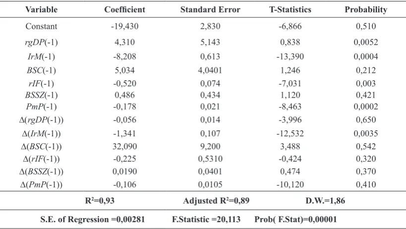
Table 5 The Results of the ARDL Model

Variable Coefficient Standard Error T-Statistics Probability

Constant -19,430 2,830 -6,866 0,510

rgDP(-1) 4,310 5,143 0,838 0,0052

IrM(-1) -8,208 0,613 -13,390 0,0004

BSC(-1) 5,034 4,0401 1,246 0,212

rIF(-1) -0,520 0,074 -7,031 0,003

BSSZ(-1) 0,486 0,434 1,120 0,421

PmP(-1) -0,178 0,021 -8,463 0,0002

D(rgDP(-1)) -0,056 0,014 -3,996 0,650

D(IrM(-1)) -1,341 0,107 -12,532 0,0035

D(BSC(-1)) 32,090 9,200 3,488 0,542

D(rIF(-1)) -0,225 0,5310 -0,424 0,320

D(BSSZ(-1)) 0,0190 0,0401 0,474 0,370

D(PmP(-1)) -0,106 0,0105 -10,120 0,410

R2_{=0,93 Adjusted R}2_{=0,89 D.W.=1,86}

S.E. of Regression =0,00281 F.Statistic =20,113 Prob( F.Stat)=0,00001

the critical value of the upper bounds at a significance level of one percent. This is an indication that the series are cointegrated. Since they are cointegrated, it means that a long-run relationship exists between them. Empirically, it suggests that a long-run relationship exists between economic growth and interest rate margin, the rate of inflation, parallel market premium, banking sector credit to the private sector and the size of the banking sector.

As seen in Table 5,

the coefficients of interest

rate margin (IrM(-1)) and D(IrM(-1)) are negative and statistically significant. The interest rate margin is a measure of the efficiency of the banking sector. The results show that both the current and previous interest rate margin are narrow. The economy is expected to grow as narrowing interest rate margin usually facilitate economic growth. In addition, the results suggest that by widening interest rate margin, it will reduce economic growth. This finding is in line with Tuuli (2002). This also confirms the theoretical positions of Blackburn and Hung (1998), and Harrison et al. (1999). These studies argue that an efficient banking system strives to eliminate or reduce the costs of the transaction by narrowing interest rate margin to encourage capital accumulation that eventually translates to economic growth.

Moreover, the coefficients of inflation (rIF (-1)) and D(rIF(-1)) are negative, but only rIF(-1) is statistically significant. The sign of the coefficient of inflation has been an issue of continuous debate in both monetary and macroeconomic literature. However, the negative sign of the coefficient of inflation supports the findings by Fischer and Modigliani (1978), and Bassey and Onwioduokit (2011).The negative sign of the coefficient of inflation means that heightening inflation is detrimental to economic growth and development. In the context of the neoclassical theory, high inflation is to reduce the value of money which causes a decline in the demand for cash, goods, and capital. This situation eventually leads to a fall in the steady state output. This is similar to the findings by Akinlo (2005), and Obamuyi and Olorunfemi (2011). However, the results can be explained in the context of the endogenous growth paradigm postulating that high inflation drastically reduces the return to deposits. This would lead to sluggish deposits accumulation behavior. The reduction in the value of return on deposits also reduces capital accumulation and output growth (Stockman, 1981).

Next, the coefficients of the current(BSSZ(-1)) and previous levels (D(BSSZ(-1)) of the size of the banking sector shows that the total of commercial banks capital plus reserves is not statistically significant. Since the total of commercial banks capital plus reserves represent the size of the banking sector implicitly meaning that the size of the banking sector during the period under consideration is not large enough to contribute to the growth of the Nigerian economy.It can also mean that size is not a potent variable of banking sector reform in Nigeria. This means that policies regulating the capital and reserves

of the commercial banks should be redesigned to enforce optimal impact on the economy.

Then, the coefficients of the previous levels of the banking sector credit to the private sector (BSC(-1)) and the change in the previous level of (D(BSC(-1))) are not statistically significant. Because the credit to the private sector is a proxy for the quality and soundness of the banking sector, it means that the volume of credit to the private sector does not correlate with the qualitative development of the sector. Furthermore, it implies that the volume of credit to the private sector is not adequate to enkindle and animate the growth of the economy. It might also mean that the balance sheet values of the credit to the private sector declared by most commercial banks in Nigeria are only a book value or unrealistic that the credit allocated and disbursed to the private sector are not used for productive economic purposes. Finally, it might mean that credit to the government is stifling and asphyxiating the growth of the private sector. Therefore, a special credit disbursement and monitoring department should be created by the apex bank to enforce effective allocation/utilization and forestall sharp practices linked to its management.

Similarly, the coefficients of parallel market premium (PmP(-1) and D(PmP(-1)) are negative and statistically insignificant. The parallel market premium is the difference between the official exchange rate and the parallel market exchange rate. The parallel market premium can be negative if there is a revaluation of the official exchange rate, and when commercial banks are restricted from buying foreign currency without proper authorization and identification. A negative parallel market premium represents a laundering charge (Dornbusch et al., 1983).

For the results of the Granger causality tests presented in Table 6 (Pesaran et al., 2001). The result of the test of causality between the rate of inflation(rIF) and economic growth (rgDP) indicates that a unidirectional causality exists between them, that is, a one-way causality runs from the rate of inflation (rIF) to economic growth (rgDP). This confirms the results of Chimobi (2010) and Barro (1995) who found a unidirectional causal linkage from inflation to economic growth.

private sector. This finding is in line with Akpasung and Babalola (2012), and Mishra et al. (2009).

Bi-directional relationships exist between parallel market premium and economic growth, and the size of the banking sector and economic growth. The causality running from economic growth to parallel market premium implies that the growth of the economy triggers the expansion of the black market. Moreover, the survival of the parallel market in Nigeria is economic growth-dependent, that is the growth of the Nigerian economy is a stimulus to the unscathed expansion and survival of the parallel

market in Nigeria. For instance, as the economy grows, the excessive demand for the exchange rate, and the consistent and persistent leakages in the official exchange rate market lead to the growth of the parallel market.In addition to that, the causality running from parallel market premium to economic growth implies that parallel market premium is critical to the growth of the Nigerian economy through faster transactions, low transaction costs, quick service delivery, smooth information flow, and total absence of time-consuming documentations.

Table 6 The Results of the Bivariate Granger Causality Tests

Economic Growth versus Inflation

Null Hypothesis

F-Statistics Direction of

Causality Decision

rgDP does not Granger cause rIF

rIF does not Granger cause rgDP

0,36 15,120*

-rIF→rgDP

Do not reject the null hypothesis Reject the null hypothesis

Economic Growth versus Banking or Financial Sector Variables

Economic Growth versus Interest Rate Margin

Null Hypothesis

F-Statistics Direction of

Causality Decision

rgDP does not Granger cause IrM

IrM does not Granger cause rgDP

0,871 27,603*

-IrM→rgDP Do not reject the null hypothesisReject the null hypothesis Economic Growth versus Banking Sector Credit to the Private Sector

Null Hypothesis

F-Statistics Direction of

Causality Decision

rgDP does not Granger cause BSC

BSC does not Granger cause rgDP

18,37* 0,77

rgDP→BSC

-Reject the null hypothesis Do not reject the null hypothesis

Economic Growth versus the Size of the Banking Sector

Null Hypothesis

F-Statistics Direction of

Causality Decision

rgDP does not Granger cause BSSZ

BSSZ does not Granger cause rgDP

36,36* 10,64*

rgDP→BSSZ

BSSZ→rgDP Reject the null hypothesisReject the null hypothesis

Economic Growth versus Parallel Market Premium

Null Hypothesis

F-Statistics Direction of

Causality Decision

rgDP does not Granger cause PmP

PmP does not Granger cause rgDP

3,76*** 9,50**

rgDP→PmP

PmP→rgDP Reject the null hypothesisReject the null hypothesis

Note: * denotes significance at the 1% level, ** at the 5% level and *** at the 10% level. All the variables are as previously defined. → denotes one-way causation.

(Source: Author’s computation using Eviews 8)

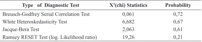
Table 7 The Result of Diagnostic Tests

Type of Diagnostic Test X2_{(chi) Statistics Probability}

Breusch-Godfrey Serial Correlation Test 0,061 0,72

White Heteroskedasticity Test 6,682 0,67

Jacque-Bera Test 2,063 0,61

Ramsey RESET Test (log. Likelihood ratio) 19,26 0,21

The result of the Breusch-Godfrey serial correlation test shown in Table 7 reveals that the probability value (0,72) is greater than 0,05 at the 95 % of the confidence interval. Therefore, it implies that the null hypothesis of the presence of serial correlation is rejected. Moreover, it can be concluded that the serial correlation is absent. This states that the covariances and the correlations between different error terms equal zero. This further means that the error terms are independently distributed implying a confirmation of the presence of serial independence. The implications of this are that the errors occurring in different periods in the model are not correlated, and there are no omitted variables, no misspecification of the model, and no systematic errors in the measurement and definition of the variables.

Furthermore, the results of White heteroskedasticity are shown in Table 7 indicating that the probability value (0,67) is greater than 0,05 at the 95% confidence interval. The researcher rejects the null hypothesis of the presence of heteroskedasticity and concludes that there is no occurrence of heteroskedasticity. This means that the disturbance terms have an equal variance or they are homoskedastic.

Meanwhile, the probability value of the JB statistic is greater than 0,05. Hence, the null hypothesis of the normality of residuals is not rejected. This indicates that the inferential statistics (F-statistic, t-statistic, and others) of this model are valid. This simply means that the residuals are normally distributed, and have zero mean and constant variance.

Finally, the empirical results of the Ramsey RESET test show that the probability value (0,21) is greater than 0,05 signifying that it does not reject the null hypothesis of a correctly specified model. Therefore, it can be concluded that the model is correctly specified. The results of all diagnostic tests such as serial correlation, heteroskedasticity, normality, and model specification tests show that the absence of serial correlation, heteroskedasticity, and the errors are normal. The Ramsey RESET test also suggests that the model is well and correctly specified.

CONCLUSIONS

This research examines the dynamic causality between banking sector reforms and economic growth in Nigeria using the ARDL bounds test for the period 1970 to 2013. Over the years, it has become obvious that the role of government such as the Presidency, the Federal Ministry of Finance and the CBN during banking sector crises has been the “crises-precipitated interventionist approach.” Banking sector reforms deserve special research attention because of the interdependence and interrelations among the banking sector, financial sector, and macroeconomic variables with implications for economic growth. The results reveal that a long-run relationship exists for the series specified in the model when economic growth

is used as the dependent variable. Reforms should be progressive( from short to medium or long-term) in banking industry stabilization programs that must be tenaciously pursued to ensure both financial and macroeconomic stability.

Concerning the causal relationship between parallel market premium and economic growth, the researcher’s recommendation is in line with Obadan (2012) and Olisadebe (1991). They opined that the parity between the official market exchange rate and the parallel market premium should be drastically reduced to accommodate transaction costs, and it should not be speculative bubbles. Furthermore, leakages from the official exchange market should be tactically curtailed as these provide incentives for the survival of the parallel market. Then, the problem of excess demand for exchange rate should be tackled to stifle the parallel market that has survived unscathed due to the persistent and consistent scarcity that is prevalent in the official exchange rate market. On a larger scale, since there are interdependence and linkages (backward and forward) within the economy, issues bordering on volatility, unpredictability, and instability occasioned by over-dependence on oil and its revenue should be tackled and settled to avoid sinister feedback effects from the real sector of the Nigerian economy to the banking sector. Meanwhile, the growth of the non-oil sector of the real economy should be stimulated and sustained to encourage capacity utilization and absorption of investment and debt. This will create a platform for the optimal utilization of the credit allocated to the private sector.

REFERENCES

Abiad, A., Detragiache, E.,& Tressel, T. (2008). A new

dataset of financial reforms. In International Monetary Fund (IMF) Working Paper.

Ajayi, M. (2005). Banking sector reforms and bank consolidation: Conceptual framework. CBN Bullion, 29(2), 2-10.

Akinlo, A. E. (2005). Impact of macroeconomic factors on total factor productivity in Sub-Saharan African countries. In Research Paper, Unu-Wider, United Nations University (UNU).

Akpansung, A. O. & Babalola, S. J. (2012).Banking sector credit and economic growth in Nigeria: An empirical investigation. Central Bank of Nigeria (CBN) Journal of Applied Statistics, 2(2), 51-62.

Andries, A. M., Apetri, A. N., & Cocris, V. (2012). The impact

of the banking system reform on banks performance. African Journal of Business Management, 6(6), 2278-2284.

Anyanwu, C. M. (2010). An overview of current banking sector reforms and the real sector of the Nigerian economy. Central Bank of Nigeria (CBN) Economic and Financial Review, 48(4), 31 - 40.

Asteriou, D.,& Hall S. G. (2007). Applied econometrics: A

Aurangzeb, C. (2012). Contributions of banking sector in

growth of Pakistan. Economics and Finance Review, 2(6), 45-54.

Awdeh, A. (2012). Banking sector development and economic growth in Lebanon. International

Research Journal of Finance and Economics, 100, 54-62.

Balogun, E. D. (2007). Banking sector reforms and the Nigerian economy: Performance, pitfalls and policy options. In Munich Personal RePEc Archive MPRA Paper (3084). University of Munich, Germany. Bassey, G. E., & Onwioduokit E. A. (2011). An analysis of

the threshold effects of inflation on economic growth

in Nigeria. West Africa Institute Financial Economic Management (WAIFEM) Review, 8(2).

Barro, R. J. (1995).Inflation and economic growth. In

National Bureau of Economic Research (NBER)

Working Paper Series.

Blackburn, K., & Hung, V. T. (1998). A theory of growth, financial development, and trade. Economica,

65(257), 107-124.

Breusch, T. S. (1978). Testing for autocorrelation in dynamic linear models. Australian Economic Papers, 17(31), 334-355.

Brissimis, S. N., Delis, M. D., & Papanikolaou, N. I. (2008). Exploring the nexus between banking sector reform and performance: Evidence from newly acceded EU countries. Journal of Banking & Finance, 32(12), 2674-2683.

CBN (2004). Central Bank of Nigeria annual report and statement of account. Retrieved from https://www. cbn.gov.ng/documents/cbnannualreports.asp

CBN (2010). Central Bank of Nigeria annual report and statement of account. Retrieved from https://www. cbn.gov.ng/documents/cbnannualreports.asp

CBN (2013). Central Bank of Nigeria annual report and statement of account. Retrieved from https://www. cbn.gov.ng/documents/cbnannualreports.asp

Chimobi, O. P. (2010). Inflation and economic growth in

Nigeria. Journal of Sustainable Development, 3(2), 159.

Dornbusch, R., Dantas, D. V., Pechman, C., de Rezende Rocha, R., & Simōes, D. (1983). The black market for Dollars in Brazil. The Quarterly Journal of

Economics, 98(1), 25-40.

Engle, R. F., & Granger, C. W. (1987). Co-integration and error correction: representation, estimation, and testing. Econometrica: Journal of the Econometric Society, 55, 251-276.

Fadare, S. O. (2010). Recent banking sector reforms and economic growth in Nigeria. Middle Eastern Finance and Economics, 8, 1450-2889.

Faruk, M. S., & Kikuchi, K. (2011). Adaptive

frequency-domain equalization in digital coherent optical

receivers. Optics Express, 19(13), 12789-12798. Faruku, A. Z., Asare, B. K., Yakubu, M., & Shehu, L. (2011).

Causality analysis of the impact of Foreign direct investment on GDP in Nigeria. Nigerian Journal of Basic and Applied Sciences, 19(1), 9-20.

Fischer, S., & Modigliani, F. (1978). Towards an understanding of the real effects and costs of

inflation. Review of World Economics, 114(4), 810-833.

Godfrey, L. G. (1978). Testing for higher order serial correlation in regression equations when the regressors include lagged dependent variables.

Econometrica: Journal of the Econometric Society, 46, 1303-1310.

Harrison, P., Sussman, O., & Zeira, J. (1999). Finance and growth: Theory and new evidence. In Federal Reserve Board Discussion Paper.

Ishioro, B. O. (2013a). Stock market development and economic growth: Evidence from Zimbabwe. Ekonomska Misao I Praksa, 22(2), 343-360.

Ishioro, B. O. (2013b). Monetary transmission mechanism in Nigeria: A Causality test. Mediterranean Journal of Social Sciences, 4(13), 377.

Ishioro, B. O. (2014). External reserves accumulation and economic growth in Nigeria: A simple Causality Test. Journal of Social and Management Sciences, 9(3), 89-101.

Ishioro, B. O. (2015).Causal relationship among economic

growth, finance, exchange rate and investment in

Nigeria. Journal of Arts and Social Sciences, 3(2), 1-21.

Ishioro, B. O. (2016). HIV/AIDS and macroeconomical

performance: Empirical evidence from Kenya. In

Scientific papers of the University of Pardubice,

Faculty of Economics and Administration.

Islam, F., Shahbaz, M., Ahmed, A. U., & Alam, M.

M. (2013). Financial development and energy consumption nexus in Malaysia: A multivariate time series analysis. Economic Modelling, 30, 435-441.

Jarque, C. M., & Bera, A. K. (1980). Efficient tests for

normality, homoscedasticity and serial independence of regression residuals. Economics letters, 6(3), 255-259.

Johansen, S. (1991). Estimation and hypothesis testing of cointegration vectors in Gaussian vector autoregressive models. Econometrica: Journal of

the Econometric Society, 59, 1551-1580.

Kama, U. (2006). Recent reforms in the Nigerian banking industry: Issues and challenges. CBN Bullion, 30(3), 65-74.

Keeley, M. C. (1990). Deposit insurance, risk, and market power in banking. The American Economic Review,

80, 1183-1200.

Keong, C. K., Yusop, Z., & Sen, V. L. K. (2005).

Export-led growth hypothesis in Malaysia: An investigation using bounds test. Sunway Academic Journal, 2, 13-22.

Khan, S., & Lewbel, A. (2007). Weighted and two-stage least squares estimation of semiparametric truncated regression models. Econometric Theory, 23(02), 309-347.

Kjosevski, J. (2013). Banking Sector Development and Economic Growth in Central and Southeastern Europe Countries. Transition Studies Review, 19(4), 461-473.

Nnanna, O. J. (2004). Beyond bank consolidation: The Impact on society. In The 4th Annual Monetary

Policy Conference of the Central Bank of Nigeria,

Abuja (18th- 19th November).

Obadan, M. I. (2012). Foreign exchange market and

the balance of payments: Elements, policies and

Nigerian experience. Benin City: Goldmark Press. Obamuyi, T. M., & Olorunfemi, S. (2011). Financial

reforms, interest rate behaviour and economic growth in Nigeria. Journal of Applied Finance and Banking, 1(4), 39-55.

Olisadebe, E. U. (1991). Appraisal of recent exchange rate policy measures in Nigeria. Central Bank of Nigeria Economic and Financial Review, 29(2), 156-185. Omotor, D. G. (2008). The role of exports in the economic

growth of Nigeria: the bounds test analysis. International Journal of Economic Perspectives, 2(4), 222-235.

Pesaran, M. H., & Shin, Y. (1998). An autoregressive distributed-lag modeling approach to cointegration analysis. Econometric Society Monographs, 31, 371-413.

Pesaran, M. H., Shin, Y., & Smith, R. J. (2001). Bounds testing approaches to the analysis of level relationships. Journal of applied econometrics,

16(3), 289-326.

Pesaran, M. H. & Smith, R. (1995). Estimating long-run relationships from dynamic heterogeneous panels. Journal of Econometrics, 68, 79-113.

Ramsey, J. B. (1969). Tests for specification errors in

Classical Linear Least-Squares Regression analysis.

Journal of the Royal Statistical Society. Series B (Methodological), 31, 350-371.

Sanusi, L. S. (2010). The Nigerian Banking Industry: what went wrong and the way forward. In Annual Convocation Ceremony of Bayero University, Kano. Sanusi, L. S. (2012). Banking reform and its impact on

the Nigerian economy. CBN Journal of Applied Statistics, 2(2), 115-122.

Simar, L., & Wilson, P. W. (2007). Estimation and inference in two-stage, semi-parametric models of production processes. Journal of Econometrics, 136(1), 31-64. Soludo, C. C. (2007). Macroeconomic, monetary and

finance sector development in Nigeria. Retrieved June 28th, 2011 from www.cenbank.org.

Stockman, A. C. (1981). Anticipated inflation and the

capital stock in a cash-in-advance economy. Journal of Monetary Economics, 8(3), 387-393.

Tuuli, K (2002). Do efficient banking sectors accelerate

economic growth in transition countries? In Bank of Finland Institute for Economies in Transition (BOFIT) Discussion Papers.

Ugwuanyi, G. O., & Amanze, P. G. (2014). Banking sector reform: An approach to restoring public confidence

on the Nigerian Banking Industry, Journal of

Finance and Accounting,5(6), 72-81.

Ugwuanyi, P. (1997). The Nigerian financial system. Enugu: Marvelous Publishers.