Article IDE implementasi model pembelajaran

(1)

Does Foreign Direct Investment

Accelerate Economic Growth?

MARIA CARKOVIC and ROSS LEVINE

195 With commercial bank lending to developing economies drying up in the 1980s, most countries eased restrictions on foreign direct investment (FDI) and many aggressively offered tax incentives and subsidies to attract for-eign capital (Aitken and Harrison 1999; World Bank 1997a, 1997b). Along with these policy changes, a surge of noncommercial bank private capital flows to developing economies in the 1990s occurred. Private capital flows to emerging-market economies exceeded $320 billion in 1996 and reached almost $200 billion in 2000. Even the 2000 figure is almost four times larger than the peak commercial bank lending years of the 1970s and early 1980s. Furthermore, FDI now accounts for over 60 percent of private capital flows. While the explosion of FDI flows is unmistakable, the growth effects remain unclear.

Theory provides conflicting predictions concerning the growth effects of FDI. The economic rationale for offering special incentives to attract FDI fre-quently derives from the belief that foreign investment produces external-ities in the form of technology transfers and spillovers. Romer (1993), for example, argues that important “idea gaps” between rich and poor countries exist. He notes that foreign investment can ease the transfer of technological

8

(2)

and business know-how to poorer countries. According to this view, FDI may boost the productivity of all firms—not just those receiving foreign capital. Thus, transfers of technology through FDI may have substantial spillover effects for the entire economy. In contrast, some theories predict that FDI in the presence of preexisting trade, price, financial, and other distortions will hurt resource allocation and slow growth (Boyd and Smith 1992). Thus, theory produces ambiguous predictions about the growth effects of FDI, and some models suggest that FDI will promote growth only under certain policy conditions.

Firm-level studies of particular countries often find that FDI does not

boost economic growth, and these studies frequently do notfind positive spillovers running between foreign-owned and domestically owned firms. Aitken and Harrison’s (1999) influential study finds no evidence of a pos-itive technology spillover from foreign firms to domestically owned ones in Venezuela between 1979 and 1989. While Blomström (1986) finds that Mexican sectors with a higher degree of foreign ownership exhibit faster productivity growth, Haddad and Harrison (1993) find no evidence of growth-enhancing spillovers in other countries. As summarized by Lipsey and Sjöholm (in this volume), in some countries, researchers find evidence of positive spillovers in some industries, but country-specific and industry-specific factors seem so important that the results do not support the over-all conclusion that FDI induces substantial spillover effects for the entire economy. In sum, firm-level studies do not imply that FDI accelerates over-all economic growth.

Unlike the microeconomic evidence, macroeconomic studies—using ag-gregate FDI flows for a broad cross section of countries—generally sug-gest a positive role for FDI in generating economic growth, especially in particular environments. For instance, Borensztein, De Gregorio, and Lee (1998) argue that FDI has a positive growth effect when the country has a highly educated workforce that allows it to exploit FDI spillovers. While Blomström, Lipsey, and Zejan (1994) find no evidence that education is crit-ical, they argue that FDI has a positive growth effect when the country is sufficiently wealthy. In turn, Alfaro et al. (2003) find that FDI promotes economic growth in economies with sufficiently developed financial mar-kets, while Balasubramanyam, Salisu, and Sapsford (1996) stress that trade openness is crucial for obtaining the growth effects of FDI.

The macroeconomic findings on growth and FDI must be viewed skep-tically, however. Existing studies do not fully control for simultaneity bias, country-specific effects, and the routine use of lagged dependent variables in growth regressions. These weaknesses can bias the coefficient estimates as well as the coefficient standard errors. Thus, the profession needs to reassess the macroeconomic evidence with econometric procedures that eliminate these potential biases.

(3)

a recent World Bank dataset (Kraay et al. 1999), we construct a panel dataset with data averaged over each of the seven five-year periods between 1960 and 1995. We also confirm the results using new FDI data from the International Monetary Fund (IMF).

Methodologically, we use the Generalized Method of Moments (GMM) panel estimator to extract consistent and efficient estimates of the impact of FDI flows on economic growth. Unlike past work, the GMM panel estima-tor exploits the time-series variation in the data, accounts for unobserved country-specific effects, allows for the inclusion of lagged dependent ables as regressors, and controls for endogeneity of all the explanatory vari-ables, including international capital flows. Thus, this study advances the literature on growth and FDI by enhancing the quality and quantity of the data and by using econometric techniques that reduce biases.

Investigating the impact of foreign capital on economic growth has important policy implications. If FDI has a positive impact on economic growth after controlling for endogeneity and other growth determinants, then this weakens arguments for restricting foreign investment. If, how-ever, we find that FDI does not exert a positive impact on growth, then this would suggest a reconsideration of the rapid expansion of tax incentives, infrastructure subsidies, import duty exemptions, and other measures that countries have adopted to attract FDI. While no single study will resolve these policy issues, this study contributes to these debates.

This study finds that the exogenous component of FDI does not exert a robust, positive influence on economic growth. By accounting for simul-taneity, country-specific effects, and lagged dependent variables as reg-ressors, we reconcile the microeconomic and macroeconomic evidence. Specifically, there is no reliable cross-country empirical evidence supporting the claim that FDI per se accelerates economic growth.

This chapter’s findings are robust to

䡲 econometric specifications that allow FDI to influence growth differ-ently depending on national income, school attainment, domestic finan-cial development, and openness to international trade;

䡲 alternative estimation procedures;

䡲 different conditioning information sets and samples;

䡲 the use of portfolio inflows instead of FDI; and

䡲 the use of alternative databases on FDI.

The data produce consistent results: there is not a robust, causal link run-ning from FDI to economic growth.

This study’s results, however, should not be viewed as suggesting that foreign capital is irrelevant for long-run growth. Borensztein, De Gregorio, and Lee (1998) show, and this study confirms, many econometric

(4)

cations in which FDI is positively linked with long-run growth. FDI may even be a positive signal of economic success as emphasized by Blomström, Lipsey, and Zejan (1994). More generally, “openness”—defined in a less narrow sense than FDI inflows—may be crucial for economic success, as suggested by other research (e.g., Bekaert, Harvey, and Lundblad 2001; Klein and Olivei 2000). Rather than examine these broad issues, this study’s contribution is much narrower: after controlling for the joint determination of growth and foreign capital flows, country-specific factors, and other growth determinants, the data do not suggest a strong independent impact of FDI on economic growth. In terms of policy implications, this study’s analyses do not support special tax breaks and subsidies to attract foreign capital. Instead, the literature suggests that sound policies encourage economic growth and also provide an attractive environment for foreign investment.

Before continuing, it is worth emphasizing this study’s boundaries. We do not discuss the determinants of FDI. Instead, we extract the exogenous component of FDI using system panel techniques. Also, we do not examine any particular country in depth. We use data on 72 countries from 1960 to 1995. Thus, our investigation provides evidence based on a cross section of countries.

Econometric Framework

This section describes two econometric methods that we use to assess the relationship between FDI inflows and economic growth. We first use sim-ple ordinary least squares (OLS) regressions with one observation per country over the 1960–95 period. Second, we use a dynamic panel proce-dure with data averaged over five-year periods, so that there are seven pos-sible observations per country between 1960 and 1995.

OLS Framework

The pure cross-sectional OLS analysis uses data averaged from 1960–95. The data include one observation per country and heteroskedasticity-consistent standard errors. The basic regression takes the form:

where the dependent variable, GROWTH, equals real per capita gross domestic product (GDP) growth, FDI is gross private capital inflows to a country, and CONDITIONING SET represents a vector of conditioning information.

(5)

Motivation for the Dynamic Panel Model

The dynamic panel approach offers advantages to OLS and also improves on previous efforts to examine the FDI-growth link using panel procedures. First, using panel data—that is, pooled cross-section and time-series data— to make estimates allows researchers to exploit the time-series nature of the relationship between FDI and growth. Thus, the panel approach included more information than the pure cross-country approach with positive ram-ifications on the precision of the coefficient estimates. Second, in a pure cross-country instrumental variable regression, any unobserved country-specific effect becomes part of the error term, which may bias the coefficient estimates (as we explain in detail below). Thus, if there are country-specific fixed effects that are not included in the conditioning set and that help explain economic growth, then the OLS procedure may produce erroneous estimates on the FDI coefficient. The panel procedures control for country-specific effects. Third, unlike existing pure cross-country studies that use instrumental variables to control for the potential endogeneity of FDI, the panel estimator controls for the potential endogeneity of allexplanatory variables. This distinction is important. If the other growth determinants besides FDI are endogenously determined with growth, which seems likely since the other growth determinants include inflation, government size, and the black market premium, among others, and if the estimation procedure does not account for this endogeneity, then this could bias FDI’s estimated coefficient and standard error. Finally, the panel estima-tor that we employ accounts explicitly for the biases induced by including initial real per capita GDP in the growth regression. Since initial real per capita GDP is a component of the dependent variable, economic growth, including this variable as a regressor may bias both the coefficient esti-mates and their standard errors, potentially leading to erroneous conclusions. For these reasons, we augment the OLS regressions with panel estimates.

Detailed Presentation of the Econometric Methodology

We use the GMM estimators developed for dynamic panel data. Our panel consists of data for a maximum of 72 countries from 1960–95, though capital flow data do not begin until 1970 for many countries. We average data over nonoverlapping, five-year periods, so that, data permitting, seven observa-tions per country (1961–65, 1966–70, etc.) are made. Thus, we exploit the time-series, along with the cross-country, dimension of the data. Consider the following regression equation:

yi t, − yi t,−1 = (α−1)yi t,−1+ ′βXi t, +ηi + εi t, ( . )8 2

(6)

where yis the logarithm of real per capita GDP, Xrepresents the set of explanatory variables (other than lagged per capita GDP), ηis an un-observed country-specific effect, εis the error term, and the subscripts iand

trepresent country and five-year time period, respectively. Specifically, X

includes FDI inflows to a country as well as other possible growth deter-minants. We also use time dummy variables for each five-year period to account for period-specific effects, though these are omitted from the equa-tions in the text. We can thus rewrite equation 8.2:

To eliminate the country-specific effect, take first differences of equation 8.3:

Thus, this eliminates potential biases associated with unobserved fixed, country effects.

Instrument variables are required to deal with both the endogeneity of all the explanatory variables and the problem that the new error term εi, t− εi, t−1,

which is correlated with the lagged dependent variable yi, t−1−yi, t−2, creates

because of the routine inclusion of lagged values of the dependent variable as a regressor. Under the assumptions that the error term is not serially correlated, and the explanatory variables are weakly exogenous (i.e., the explanatory variables are uncorrelated with future realizations of the error term), the GMM dynamic panel estimator uses the following moment con-ditions, where sand tindicate the five-year period under evaluation:

We refer to the GMM estimator based on these conditions as the difference estimator.

There are, however, conceptual and statistical shortcomings with this difference estimator. Conceptually, we would also like to study the cross-country relationship between financial development and per capita GDP growth, which is eliminated in the difference estimator. When the explana-tory variables are persistent over time, lagged levels make weak instru-ments for the regression equation in first differences. Instrument weakness influences the asymptotic and small-sample performance of the difference estimator. Asymptotically, the variance of the coefficients rises. In small samples, weak instruments can bias the coefficients.

To reduce the potential biases and imprecision associated with the usual estimator, we use a new estimator that combines in a system the regression in differences with the regression in levels. The instruments for the

regres-E X i t s,− 䡠(εi t, −εi t,−1) = 0 for s≥ 2;t = 3, . . . ,T ( . )8 5 E y i t s,− 䡠(εi t, −εi t,−1) = 0 for s ≥ 2;t = 3, . . . ,T ( . )8 4 yi t, − yi t,−1 = α(yi t,−1− yi t,−2)+ ′β(Xi t, −Xi t,−1)+(εi t, −εi t,−1)

(7)

sion in differences are the same as above. The instruments for the regres-sion in levels are the lagged differences of the corresponding variables. These are appropriate instruments under the following additional assump-tion: although there may be correlation between the levels of the right-hand variables and the country-specific effect in equation 8.3, there is no cor-relation between the differences of these variables and the country-specific effect. The following equation specifies this more formally, where

p, q, and tindicate time periods:

The additional moment conditions for the second part of the system (the regression in levels) are:

Thus, we use the moment conditions presented in equations 8.4, 8.5, 8.7, and 8.8, use instruments lagged two periods (t−2), and employ a GMM pro-cedure to generate consistent and efficient parameter estimates.1

Consistency of the GMM estimator depends on the validity of the instru-ments. To address this issue we consider two specification tests. The first is a Sargan test of overidentifying restrictions, which tests the overall validity of the instruments by analyzing the sample analog of the moment conditions used in the estimation process. The second test examines the hypothesis that the error term εi, tis not serially correlated. In both the difference regression

E X( i t s,− −Xi t s,− −1)䡠(ηi +εi t,) = 0 for s= 1 ( . )8 8 E y( i t s,− −yi t s,− −1)䡠(ηi +εi t,) = 0 for s= 1 ( . )8 7 E y E y and E X E X

for all p and q

i t p, i i t q, i i t p, i i t q, i

( . )

+ + + +

 䡠η =  䡠η  䡠η =  䡠η

8 6

DOES FDI ACCELERATE ECONOMIC GROWTH? 201

1. We use a variant of the standard two-step system estimator that controls for het-eroskedasticity. Typically, the system estimator treats the moment conditions as applying to a particular time period. This provides for a more flexible variance-covariance structure of the moment conditions because the variance for a given moment condition is not assumed to be the same across time. The drawback of this approach is that the number of overidentifying conditions increases dramatically as the number of time periods increases. Consequently, this typical two-step estimator tends to induce overfitting and potentially biased standard errors. To limit the number of overidentifying conditions, we follow Beck and Levine (2003) by applying each moment condition to all available periods. This reduces the overfitting bias of the two-step estimator. However, applying this modified estimator reduces the number of periods by one. While in the standard estimator time dummies and the constant are used as instruments for the second period, this modified estimator does not allow the use of the first and second periods. We confirm the results using the standard system estimator.

(8)

and the system difference–level regression, we test whether the differenced error term is second-order serially correlated (by construction, the differ-enced error term is probably first-order serially correlated even if the origi-nal error term is not).

The panel procedure also has disadvantages and limitations. The major disadvantage relative to a pure cross-country comparison is that this study focuses on economic growth and seeks to abstract from business cycles and crises. To use panel procedures, however, the data are averaged over five-year periods, which may not eliminate higher frequency forces. Thus, to assess the robustness of the results, we employ both OLS techniques that use data averaged over more than 35 years and panel techniques that use data averaged over five-year periods. Furthermore, the panel procedure has lim-itations in that it does not solve all of the problems associated with cross-country regressions. For instance, FDI may have complex dynamic effects, such that the impact of FDI is different from the short run to the long run. We provide some sensitivity checks along this dimension by presenting results based on data averaged over both 35 years and 5 years. Nevertheless, this study does not attempt to trace the potential time-varying effects of FDI on growth. Finally, this study provides an aggregate examination. While a mul-titude of firm-level and industry-level studies of FDI exist, in particular coun-tries that attempt to assess the effects of specific policies (see the chapters by Moran as well as Lipsey and Sjöholm in this volume), this study undertakes a general assessment of the relationship between FDI and growth.

Data

We collected FDI data from two sources. First, we use data from the World Bank’s ongoing project to improve the accuracy, breadth, and length of national accounts data (Kraay et al. 1999). Second, we confirm the findings using the IMF’s World Economic Output(2001) data on openness. We now define each variable.

䡲 FDIequals gross FDI inflows as a share of GDP. We confirm the results using FDI inflows per capita.2

䡲 GROWTHequals the rate of real per capita GDP growth.

(9)

To assess the link between international capital flows and economic growth and its sources, we control for other growth determinants: Initial income per capitaequals the logarithm of real per capita GDP at the start of each period, so that it equals 1960 in the pure cross-country analyses and, thereafter, the first year of each five-year period in the panel estimates.

Average years of schoolingequals the average years of schooling of the working-age population. Inflationequals the average growth rate in the consumer price index. Government sizeequals the size of the government as a share of GDP.

Openness to tradeequals exports plus imports relative to GDP. Black market premiumequals the black market premium in the foreign exchange market.

Private creditequals credit by financial intermediaries to the private sector as a share of GDP (Beck, Levine, and Loayza 2000).

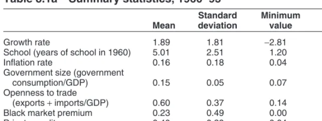
Tables 8.1a and 8.1b present summary statistics and correlations using data averaged over the 1960–95 period, with one observation per country. There is considerable cross-country variation. For instance, the mean per capita growth rate for the sample is 1.9 percent per annum, with a standard deviation of 1.8. The maximum growth rate was enjoyed by South Korea (7.2), while Niger and Zaire suffered with a per capita growth rate of worse than −2.7 percent per annum. In the five-year periods, the minimum value is −10.0 percent growth (Rwanda 1990–95), and a number of countries expe-rienced five-year growth spurts of greater than 8 percent per annum. The data also suggest large variation in FDI with the average of 1.1 percent of GDP. Malaysia as well as Trinidad and Tobago had FDI inflows of more than 3.6 percent of GDP over the entire 1960–95 time period, while Sudan essentially had no FDI over this period. In terms of five-year periods, the maximum value of FDI was 7.3 percent of GDP (in Malaysia from 1990–95). The variability over five-year periods is much larger than when using lower-frequency data. Although tables 8.1a and 8.1b do not suggest a simple, pos-itive relationship between FDI and growth, we will see that many growth regression specifications yield a positive coefficient on FDI.

Results

This study estimates the effects of FDI inflows on economic growth after controlling for other growth determinants and the potential biases induced by endogeneity, country-specific effects, and the inclusion of initial income as a regressor. Moreover, we examine whether the growth effects of FDI depend on the recipient country’s level of educational attainment, eco-nomic development, financial development, and trade openness.

Findings

Table 8.2 shows that the exogenous component of FDI does not exert a reli-able, positive impact on economic growth. The table presents OLS and panel

(10)

estimates using a variety of conditioning information sets. In the OLS regres-sions, initial income and average years of schooling enter significantly and with the signs and magnitudes found in many pure cross-country regres-sions. FDI does not enter these growth regressions significantly. When we move to the five-year panel data, FDI enters three of the regressions signifi-cantly but not the other four. FDI enters the regressions signifisignifi-cantly and pos-itively in the regression that includes only initial income per capita and average years of schooling as control variables. FDI remains significantly and positively linked with growth when controlling for inflation or govern-ment size. However, FDI becomes insignificant once we control for trade openness, the black market premium, or financial development. In sum, FDI is never significant in the OLS regressions and becomes insignificant in the panel estimation when controlling for financial development or when con-trolling for international openness as proxied by either the trade share or the black market premium.3

Furthermore, the coefficient on FDI is unstable in the panel regressions, ranging from 323 (when controlling for initial income, schooling, and infla-tion) to −34 (when controlling for initial income, schooling, and financial development). Changes in the sample do not cause this instability. When the regressions are restricted to have the same number of observations, the

Table 8.1a Summary statistics, 1960–95

Standard Minimum Maximum

Mean deviation value value

Growth rate 1.89 1.81 −2.81 7.16

School (years of school in 1960) 5.01 2.51 1.20 11.07

Inflation rate 0.16 0.18 0.04 0.91

Government size (government

consumption/GDP) 0.15 0.05 0.07 0.31

Openness to trade

(exports +imports/GDP) 0.60 0.37 0.14 2.32

Black market premium 0.23 0.49 0.00 2.77

Private credit 0.40 0.29 0.04 1.41

FDI (as a share of GDP) 0.011 0.010 0.000 0.043

(11)

205

Table 8.1b Correlation matrix, 1960–95

Openness Black-market Private Growth Schoola _Inflationb _{Government size}a _{to trade}b _premiumb _credita _FDI

Growth 1

Average years of schoolinga _0.45* ₁

Inflationb −_0.28* −_0.08 ₁

Government sizea _0.24* _0.42* ₋_0.28* ₁

Openness to tradea _0.21 _0.04 −_0.36* _0.33* ₁

Black-market premiumb ₋_0.43* ₋_0.40* _0.38* ₋_0.20 _0.07 ₁

Private credita _0.55* _0.68* −_0.43* _0.39* _0.03 −_0.60* ₁

FDI 0.17 0.12 −0.21 0.23 0.56* −0.01 0.05 1

* =indicates significance at the 0.05 level.

Note: This table is based on a common sample of 64 countries using the average between 1960 and 1995, with one observation per country.

(12)

coefficient on FDI remains unstable.4_{Note that the Sargan and serial}

cor-relation tests do not reject the econometric specification. The table 8.2 regressions do not reject the null hypothesis that FDI does not exert an independent influence on economic growth.

We also assess whether the impact of FDI on growth depends heavily on the stock of human capital (table 8.3). Borensztein, De Gregorio, and Lee (1998) find that in countries with low levels of human capital the direct effect of FDI on growth is negative, though sometimes insignificant. But once human capital passes a threshold, they find that FDI has a positive growth effect. The rationale is that only countries with sufficiently high levels of human capital can exploit the technological spillovers associated with FDI. Thus, we include the interaction term FDI*School, which equals the product of FDI and the average years of schooling of the working-age population.

Table 8.3 shows that the lackof FDI impact on growth does not depend on the stock of human capital. In the OLS regressions, FDI and the interac-tion term do not enter significantly in any of the six regressions. In the panel regressions, FDI and the interaction term occasionally enter significantly, but even here the results do not conform to theory. Namely, when FDI and the interaction term do enter significantly, the term on FDI is significant and the coefficient on the interaction term is negative. This suggests that FDI is only growth enhancing in countries with low educational attainment. These counterintuitive results may result from including schooling, FDI, and the interaction term simultaneously.5_{When excluding schooling, however,}

the regressions do not yield robust results with a positive coefficient on the interaction term.

Finally, we also examined the importance of human capital using an alter-native specification. Instead of including the interaction term FDI*School, we created a dummy variable, D, that takes on the value 1 if the country has greater than average schooling and 0 otherwise. We then included the term FDI*D. This specification also indicated that FDI’s impact on growth

4. Also, note that the coefficient on FDI is frequently, though not always, an order of magni-tude larger in the panel than the OLS regressions. We speculate that this occurs because of more volatile data. When we restrict the sample to wealthier countries (which are also coun-tries with less volatile growth rates), the panel coefficient on FDI is similar to the OLS regres-sion coefficients. Similarly, when we use the IMF’s World Economic Outlookdata, which contains fewer and very poor, highly volatile countries than the World Bank data, the panel coefficients are closer to the coefficients from the OLS regressions. These estimates are con-sistent with the view that short-run fluctuations in the investment environment, and hence FDI, are associated with large, though temporary, booms and busts in economic performance. Thus, the use of higher frequency data produces larger (though still insignificant) coefficients on FDI than pure cross-country regressions with data averaged over the 1960–95 period.

(13)

Table 8.2 Growth and FDI regressions, 5-year periods 1960–95

1 2 3 4 5 6 7

OLS Panel OLS Panel OLS Panel OLS Panel OLS Panel OLS Panel OLS Panel

Constant 6.797 −0.723 7.732 9.324 7.363 −10.640 6.222 5.646 7.103 2.391 11.579 5.256 11.702 2.701

(0.009) (0.896) (0.002) (0.314) (0.015) (0.303) (0.074) (0.259) (0.006) (0.716) (0.000) (0.332) (0.000) (0.668)

Initial income −1.175 −0.252 −1.226 −3.026 −1.274 −1.522 −1.236 0.233 −1.191 −0.667 −1.414 0.720 −1.643 −0.508 per capitaa _(0.008) _{(0.854) (0.003)} _(0.254) _(0.005) _(0.500) _{(0.006) (0.822)} _(0.007) _{(0.708) (0.000)} _(0.415) _{(0.000) (0.679)}

Average years 2.752 2.551 2.774 8.629 2.979 6.770 2.934 0.096 2.661 2.480 1.840 −2.576 2.115 1.617

of schoolingb _(0.000) _{(0.407) (0.000)} _(0.182) _(0.000) _(0.195) _{(0.000) (0.967)} _(0.001) _{(0.556) (0.003)} _(0.230) _{(0.001) (0.696)}

Inflationb −_3.377 −_0.887 _1.398 −_0.161

(0.034) (0.839) (0.355) (0.949)

Government sizea ₋_0.083 ₋_6.461 ₋_0.854 ₋_2.796

(0.878) (0.060) (0.127) (0.165)

Openness to tradea _0.193 _4.830 _0.427 _1.664

(0.650) (0.000) (0.329) (0.375)

Black market premiumb ₋_0.292 ₋_0.590 ₋_1.028 ₋_1.505

(0.792) (0.645) (0.272) (0.285)

Private-sector creditb _1.397 _2.262 _1.714 _1.250

(0.000) (0.027) (0.001) (0.333)

FDI 12.553 202.167 2.852 322.933 16.598 215.245 10.677 17.045 12.558 220.854 14.854 −34.511 21.931 −9.434

(0.582) (0.006) (0.897) (0.051) (0.469) (0.049) (0.631) (0.748) (0.579) (0.160) (0.414) (0.609) (0.238) (0.917)

Conditioning information set

(table continues next page)

(14)

Table 8.2 Growth and FDI regressions (continued)

1 2 3 4 5 6 7

OLS Panel OLS Panel OLS Panel OLS Panel OLS Panel OLS Panel OLS Panel

Number of observationsc ₆₈ ₂₇₉ ₆₈ ₂₇₀ ₆₈ ₂₇₃ ₆₇ ₂₇₇ ₆₆ ₂₆₀ ₆₇ ₂₄₆ ₆₄ ₂₄₂

R2_(adjusted) _0.238 _0.287 _0.238 _0.258 _0.209 _0.437 _0.510

Sargan test (p-value)d _0.098 _0.770 _0.756 _0.299 _0.302 _0.304 _0.191

Serial correlation

test (p-value)e _0.939 _0.922 _0.897 _0.580 _0.805 _0.234 _0.256

OLS = ordinary least squares

a. In the regression, this variable is included as Ln(variable). b. In the regression, this variable is included as Ln(1 +variable). c. Panel estimations use five-year periods.

d. The null hypothesis is that the instruments are not correlated with the residuals.

e. The null hypothesis is that the errors in the first-difference regression exhibit no second-order serial correlation.

Notes: Dependent variable is real per capita GDP growth. P-values are in parentheses below estimates’ coefficient values.

(15)

Table 8.3 Growth, FDI, and education regressions

1 2 3 4 5 6

OLS Panel OLS Panel OLS Panel OLS Panel OLS Panel OLS Panel

Constant 6.841 1.504 7.727 11.765 7.312 −21.189 6.050 6.882 7.250 −3.460 6.812 −4.611

(0.011) (0.857) (0.003) (0.252) (0.017) (0.120) (0.093) (0.179) (0.007) (0.651) (0.029) (0.513)

Initial income −1.175 −1.484 −1.226 −4.718 −1.281 −2.346 −1.238 −0.625 −1.190 −0.631 −1.391 −3.843 per capitaa _(0.008) _(0.451) _(0.003) _(0.091) _(0.005) _(0.295) _(0.007) _(0.593) _(0.007) _(0.738) _(0.002) _(0.012)

Average years 2.721 7.025 2.778 15.183 3.120 12.607 3.052 2.612 2.557 5.520 3.415 14.161

of schoolingb _(0.001) _(0.111) _(0.000) _(0.026) _(0.002) _(0.015) _(0.000) _(0.341) _(0.006) _(0.191) _(0.001) _(0.000)

Inflationb ₋_3.378 ₋_2.783 ₋_3.812 ₋_6.959

(0.035) (0.586) (0.052) (0.026)

(0.837) (0.015) (0.388) (0.013)

Openness to tradea _0.199 _4.012 ₋_0.078 _1.706

(0.644) (0.005) (0.871) (0.440)

Black market −0.314 0.690 0.037 2.256

premiumb _(0.782) _(0.549) _(0.977) _(0.014)

FDI 7.585 471.575 3.460 567.935 35.139 588.334 28.284 155.478 −2.463 681.882 46.078 351.000

(0.901) (0.010) (0.953) (0.028) (0.604) (0.004) (0.618) (0.040) (0.970) (0.000) (0.485) (0.000)

FDI*School 3.350 −183.992 −0.411 −161.501 −12.179 −250.233 −11.905 −48.640 10.084 −243.945 −23.042 −108.606 (0.935) (0.036) (0.992) (0.198) (0.785) (0.063) (0.756) (0.232) (0.817) (0.000) (0.606) (0.014)

(table continues next page)

(16)

Table 8.3 Growth, FDI, and education regressions (continued)

1 2 3 4 5 6

Number of

observationsc ₆₈ ₂₇₉ ₆₈ ₂₇₀ ₆₆ ₂₇₃ ₆₇ ₂₇₇ ₆₆ ₂₆₀ ₆₅ ₂₄₈

R2_(adjusted) _0.226 _0.275 _0.226 _0.247 _0.197 _0.258

Sargan test (p-value)d _0.340 _0.690 _0.828 _0.286 _0.324 _0.144

Serial correlation test

(p-value)e _0.332 _0.506 _0.273 _0.283 _0.158 _0.221

(17)

DOES FDI ACCELERATE ECONOMIC GROWTH? 211 does not robustly vary with the level of educational attainment. While some may interpret the results in table 8.3 as suggesting that the coefficient on FDI becomes significant and positive in the panel regressions when con-trolling for the interaction with schooling, we note that (1) the interaction terms are frequently insignificant, (2) the signs do not conform with theory, and (3) the OLS regressions suggest a fragile relationship.

Since Blomström, Lipsey, and Zejan (1994) argue that very poor coun-tries—countries that are extremely technologically backward—are unable to exploit FDI, we reran the regressions using the interaction term, FDI*Income per capita. Table 8.4 shows, however, that a reliable link between growth and FDI when allowing for FDI’s impact on growth to depend on the level of income per capita does not exist.6

Table 8.5 assesses whether the level of financial development in the recip-ient country influences the growth-FDI relationship. Better-developed financial systems improve capital allocation and stimulate growth (Beck, Levine, and Loayza 2000). Capital inflows to a country with a well-developed financial system may, therefore, produce substantial growth effects. Thus, we reran the regressions using the interaction term FDI*Credit.

Although the OLS regressions in table 8.5 suggest that FDI has a positive growth effect, especially in financially developed economies, the panel evi-dence does not confirm this finding. The panel regressions never demon-strated a significant coefficient on the FDI-financial development interaction term. On net, these results do not provide much support for the view that FDI flows to financially developed economies exert an exogenous impact on growth.

Table 8.6 assesses whether the relationship between FDI and growth varies with the degree of trade openness. Balasubramanyam, Salisu, and Sapsford (1996, 1999) find evidence that FDI is particularly good for eco-nomic growth in countries with open trade regimes. Thus, we include an interaction term of FDI and openness to trade in the table 8.6 regressions. The FDI*Trade interaction term does not enter significantly in any of the OLS regressions. While the FDI*Trade interaction term enters significantly at the 0.10 level in three of the panel regressions, it enters insignificantly in the other three. In sum, we do not find a robust link between FDI and growth even when allowing this relationship to vary with trade openness. While FDI flows may go hand in hand with economic success, they do not tend to exert an independent growth effect. Thus, by correcting statistical

(18)

Table 8.4 Growth, FDI, and income level regressions

1 2 3 4 5 6

Constant 4.609 −5.254 5.623 8.400 5.263 −15.806 4.493 4.792 5.029 −4.906 3.765 −3.550

(0.209) (0.459) (0.102) (0.446) (0.167) (0.213) (0.293) (0.410) (0.178) (0.562) (0.368) (0.675)

Initial income −0.880 0.320 −0.942 −3.356 −0.939 −1.638 −0.961 −0.247 −0.918 −0.113 −1.002 −1.340 per capitaa _(0.115) _(0.837) _(0.071) _(0.225) _(0.101) _(0.457) _(0.090) _(0.829) _(0.100) _(0.952) _(0.072) _(0.315)

Average years 2.698 2.731 2.723 10.933 2.998 8.922 2.901 2.240 2.635 4.043 3.205 6.488

of schoolingb _(0.000) _(0.377) _(0.000) _(0.075) _(0.000) _(0.057) _(0.000) _(0.391) _(0.001) _(0.327) _(0.000) _(0.018)

Inflationb ₋_3.354 ₋_2.248 ₋_4.078 ₋_4.433

(0.034) (0.609) (0.034) (0.124)

Government sizea −_0.282 −_7.663 −_0.662 −_4.512

(0.627) (0.029) (0.288) (0.090)

Openness to tradea _0.100 _4.034 ₋_0.239 _2.918

(0.813) (0.005) (0.618) (0.173)

Black market −0.232 0.893 0.127 1.105

premiumb _(0.840) _(0.572) _(0.920) _(0.257)

(19)

FDI 224.576 610.123 206.638 664.202 268.111 669.822 226.791 254.810 209.550 1114.655 322.879 311.729 (0.265) (0.055) (0.289) (0.149) (0.219) (0.178) (0.245) (0.421) (0.312) (0.030) (0.131) (0.137)

FDI*Income −27.398 −53.443 −26.325 −46.457 −32.294 −56.910 −27.567 −22.900 −25.438 −110.359 −39.591 −30.888

per capita (0.257) (0.202) (0.262) (0.463) (0.219) (0.385) (0.241) (0.607) (0.307) (0.043) (0.125) (0.312)

Number of

observationsc ₆₈ ₂₇₉ ₆₈ ₂₇₀ ₆₅ ₂₇₃ ₆₇ ₂₇₇ ₆₆ ₂₆₀ ₆₅ ₂₄₈

R2_(adjusted) _0.237 _0.286 _0.240 _0.257 _0.206 _0.367

Serial correlation

test (p-value)e _0.553 _0.871 _0.935 _0.680 _0.405 _0.587

(20)

Table 8.5 Growth, FDI, and finance regressions

1 2 3 4 5 6

Constant 9.236 4.453 9.380 −7.651 9.609 −4.337 8.887 8.217 9.454 0.383 9.119 −4.088

(0.000) (0.592) (0.000) (0.146) (0.001) (0.508) (0.007) (0.094) (0.000) (0.935) (0.001) (0.627)

Initial income −1.407 −0.724 −1.401 1.498 −1.479 1.780 −1.460 −0.743 −1.397 0.624 −1.465 −0.650

per capitaa _(0.000) _(0.712) _(0.000) _(0.215) _(0.000) _(0.235) _(0.001) _(0.453) _(0.001) _(0.620) _(0.001) _(0.723)

Average years 2.294 2.087 2.358 −0.596 2.483 −1.910 2.477 2.637 2.162 −1.030 2.503 3.060

of schoolingb _(0.000) _(0.630) _(0.000) _(0.813) _(0.001) _(0.550) _(0.000) _(0.240) _(0.002) _(0.746) _(0.001) _(0.458)

Inflationb ₋_1.730 ₋_2.584 ₋_1.118 ₋_2.123

(0.222) (0.197) (0.464) (0.475)

Government sizea −_0.061 _1.600 −_0.325 −_4.397

(0.911) (0.326) (0.573) (0.071)

Openness to tradea _0.114 _4.448 _0.155 _0.506

(0.753) (0.001) (0.714) (0.824)

Black market −0.732 −4.589 −1.162 −3.900

premiumb _(0.336) _(0.062) _(0.100) _(0.034)

(21)

FDI 152.323 −340.106 133.016 71.044 152.237 −107.266 147.760 −40.957 141.844 −237.720 119.251 −300.341 (0.000) (0.222) (0.000) (0.624) (0.000) (0.431) (0.000) (0.775) (0.001) (0.263) (0.000) (0.046)

FDI*Credit 123.541 136.398 110.615 −8.229 120.562 41.469 119.495 33.787 113.364 62.675 93.643 84.242

(0.000) (0.100) (0.000) (0.855) (0.000) (0.347) (0.000) (0.429) (0.000) (0.218) (0.001) (0.133)

Number of

observationsc ₆₇ ₂₆₉ ₆₇ ₂₆₄ ₆₅ ₂₆₃ ₆₆ ₂₆₇ ₆₅ ₂₅₀ ₆₄ ₂₄₂

R2_(adjusted) _0.441 _0.447 _0.442 _0.456 _0.432 _0.451

Serial correlation

test (p-value)e _0.787 _0.992 _0.206 _0.356 _0.213 _0.145

(22)

Table 8.6 Growth, FDI, and trade openness regressions

1 2 3 4 5 6

Constant 6.462 4.531 7.563 10.971 5.700 −0.876 6.366 5.419 6.935 6.620 6.336 2.524

(0.018) (0.478) (0.004) (0.255) (0.055) (0.918) (0.020) (0.330) (0.011) (0.376) (0.027) (0.706)

Initial income −1.135 −1.120 −1.230 −3.168 −1.114 −2.698 −1.137 −0.216 −1.151 −1.393 −1.270 −5.637 per capitaa _(0.013) _(0.482) _(0.004) _(0.242) _(0.018) _(0.257) _(0.014) _(0.863) _(0.012) _(0.504) _(0.005) _(0.005)

Average years 2.812 5.182 2.878 9.036 2.847 9.223 2.806 2.519 2.659 4.603 2.991 16.644

of schoolingb _(0.000) _(0.155) _(0.000) _(0.187) _(0.000) _(0.100) _(0.000) _(0.413) _(0.001) _(0.373) _(0.000) _(0.001)

Inflationb −_3.057 −_2.353 −_3.609 −_9.122

(0.061) (0.529) (0.065) (0.014)

(0.598) (0.084) (0.354) (0.005)

Openness to tradea −_0.152 _4.869 −_0.442 −_3.553

(0.734) (0.001) (0.369) (0.068)

Black market −0.605 −1.823 −0.139 0.555

premiumb _(0.654) _(0.176) _(0.919) _(0.625)

(23)

FDI 16.430 150.596 7.310 234.048 17.881 201.450 20.850 75.550 16.894 99.801 22.961 236.671 (0.458) (0.041) (0.746) (0.106) (0.435) (0.037) (0.473) (0.109) (0.417) (0.504) (0.424) (0.009)

FDI*Trade 29.241 259.748 17.771 56.605 33.007 217.435 35.456 89.843 33.880 148.279 39.920 324.020

(0.491) (0.001) (0.670) (0.626) (0.445) (0.053) (0.479) (0.162) (0.370) (0.237) (0.361) (0.008)

Number of

observationsc ₆₇ ₂₇₆ ₆₇ ₂₆₇ ₆₆ ₂₇₀ ₆₇ ₂₇₅ ₆₅ ₂₅₇ ₆₅ ₂₄₅

R2_(adjusted) _0.269 _0.305 _0.241 _0.258 _0.249 _0.270

Serial correlation

test (p-value)e _0.318 _0.940 _0.996 _0.443 _0.985 _0.667

(24)

shortcomings with past work this study reconciles the broad cross-country evidence with microeconomic studies.

Sensitivity Analyses

We conduct a number of sensitivity analyses to assess the robustness of the results. First, we use a standard instrumental variable estimator in a pure cross-country context (one observation per country) and reexamine whether country variations in the exogenous component of FDI explain cross-country variations in the rate of economic growth. We use GMM.7_{We also}

use linearmoment conditions, which amounts to the requirement that the instrumental variables (Z) are uncorrelated with the error term in the growth regression in equation 8.1. The economic meaning of these conditions is that the instrumental variables can only affect growththrough FDI and the other variables in the conditioning information set. To test this condition, we test the overidentifying restrictions, and we cannot reject the given moment con-ditions. The GMM results confirm this study’s results.

Second, we confirm this study’s findings using two alternative estima-tors. Instead of using Calderon, Chong, and Loayza’s (2000) method of lim-iting the possibility of overfitting by restricting the dimensionality of the instrument set (described above), we use the standard system estimator. In addition, although the standard estimator and Calderon, Chong, and Loayza’s (2000) modification are two-step estimators where the variance-covariance matrix is constructed from the first-stage residuals to allow for nonspherical distributions of the error term (and thereby get more efficient estimates in the second stage), these two-step GMM estimators sometimes converge to their asymptotic distributions slowly. This tends to bias the t-statistics upward. Nonetheless, we reran the regressions using the first-stage results, which assume homoskedasticity and independence of the error terms.

Third, we used a variety of alternative samples and specifications. As noted by Blonigen and Wang (in this volume), there may be concerns about mixing rich and poor countries in empirical studies of FDI and growth. Nonetheless, limiting the sample to developing countries—i.e., countries not classified by the World Bank as high-income economies—does not alter the findings. Also, when using a common sample across all of the regres-sions, the results do not change. Similarly, using the natural logarithm of FDI does not alter the conclusions. We also considered exchange rate volatil-ity, changes in the terms of trade in the regression, and various combinations of the conditioning information set (Levine and Renelt 1992). Including these factors did not alter the conclusions. This study does not prove that FDI is unimportant. Rather, this cross-country analysis—in conjunction with

(25)

microeconomic evidence—reduces confidence in the belief that FDI acceler-ates GDP growth.

Fourth, we examined whether FDI affects productivity growth using the Easterly and Levine (2001) measure of total factor productivity (TFP). We found that FDI does not exert a robust impact on TFP.

Fifth, we examined portfolio inflows and found that they do not have a positive impact on growth.

Finally, we repeated the analyses using the IMF’s World Economic Outlook 2001new database on international capital flows. The IMF cleaned the data and extended the findings through the end of 2000. The results are very similar to those reported above, so we do not report them.

Conclusion

FDI has increased dramatically since the 1980s. Furthermore, many coun-tries have offered special tax incentives and subsidies to attract foreign cap-ital. An influential economic rationale for treating foreign capital favorably is that FDI and portfolio inflows encourage technology transfers that accel-erate overall economic growth in recipient countries. While microeconomic studies generally, though not uniformly, shed pessimistic evidence on the growth effects of foreign capital, many macroeconomic studies find a posi-tive link between FDI and growth. Previous macroeconomic studies, how-ever, do not fully control for endogeneity, country-specific effects, and the inclusion of lagged dependent variables in the growth regression.

After resolving many of the statistical problems plaguing past macroeco-nomic studies and confirming our results using two new databases on inter-national capital flows, we find that FDI inflows do not exert an independent influence on economic growth. Thus, while sound economic policies may spur both growth and FDI, the results are inconsistent with the view that FDI exerts a positive impact on growth that is independent of other growth determinants.

References

Aitken, Brian, and Ann Harrison. 1999. Do Domestic Firms Benefit from Foreign Direct In-vestment? Evidence from Venezuela. American Economic Review89, no. 3 (June): 605–18. Alfaro, Laura, Chanda Areendam, Sebnem Kalemli-Ozcan, and Sayek Selin. 2003. FDI and Economic Growth: The Role of Local Financial Markets. Journal of International Economics

61, no. 1 (October): 512–33.

Balasubramanyam, V. N., Mohammed Salisu, and David Sapsford. 1996. Foreign Direct Investment and Growth in EP and IS Countries. Economic Journal106, no. 434 (January): 92–105.

Balasubramanyam, V. N., Mohammed Salisu, and David Sapsford. 1999. Foreign Direct Invest-ment as an Engine of Growth. Journal of International Trade and Economic Development8, no. 1: 27–40.

(26)

Beck, Thorsten, and Ross Levine. 2003. Stock Markets, Banks, and Growth: Panel Evidence.

Journal of Banking and Finance28, no. 3 (March): 423–42.

Beck, Thorsten, Ross Levine, and Norman Loayza. 2000. Finance and the Sources of Growth.

Journal of Financial Economics58, no. 1-2: 261–300.

Bekaert, Geert, Campbell R. Harvey, and Christian Lundblad. 2001. Does Financial Liberalization Spur Growth?NBER Working Paper 8245. Cambridge, MA: National Bureau of Economic Research.

Blomström, Magnus. 1986. Foreign Investment and Productive Efficiency: The Case of Mexico. The Journal of Industrial Economics35, no. 1 (April): 97–110.

Blomström, Magnus, Robert E. Lipsey, and Mario Zejan. 1994. What Explains Developing Country Growth? In Convergence and Productivity: Gross-National Studies and Historical Evidence,ed. William Baumol, Richard Nelson, and Edward Wolff. Oxford: Oxford University Press.

Borensztein, E., J. De Gregorio, and J. W. Lee. 1998. How Does Foreign Investment Affect Growth? Journal of International Economics45, no. 1: 115–72.

Boyd, John H., and Bruce D. Smith. 1992. Intermediation and the Equilibrium Allocation of Investment Capital: Implications for Economic Development. Journal of Monetary Economics30: 409–32.

Calderon, Cesar, Alberto Chong, and Norman Loayza. 2000. Determinants of Current Account Deficits in Developing Countries.World Bank Research Policy Working Paper 2398 (July). Washington: World Bank.

Easterly, William, and Ross Levine. 2001. It’s Not Factor Accumulation: Stylized Facts and Growth Models. World Bank Economic Review15: 177–219.

Haddad, Mona, and Ann Harrison. 1993. Are There Positive Spillovers from Direct Foreign Investment? Evidence from Panel Data for Morocco. Journal of Development Economics42 (October): 51–74.

Klein, Michael, and Giovanni Olivei. 2000. Capital Account Liberalization, Financial Depth, and Economic Growth. Somerville, MA: Tufts University. Photocopy.

Kraay, Aart, Norman Loayza, Luis Serven, and Jaime Ventura. 1999. Country Portfolios. Washington: World Bank. Photocopy.

La Porta, Rafael, Florencio Lopez-de-Silanes, Andrei Shleifer, and Robert W. Vishny. 1999. The Quality of Government. Journal of Law, Economics, and Organization15, no. 1: 222–79. Levine, Ross, and Maria Carkovic. 2001. How Much Bang for the Buck: Mexico and

Dollarization. Journal of Money, Credit, and Banking33, no. 2 (May): 339–63.

Levine, Ross, Norman Loayza, and Thorsten Beck. 2000. Financial Intermediation and Growth: Causality and Causes. Journal of Monetary Economics46: 31–77.

Levine, Ross, and David Renelt. 1992. A Sensitivity Analysis of Cross-Country Growth Regressions. American Economic Review82, no. 4 (September): 942–63.

Romer, Paul. 1993. Idea Gaps and Object Gaps in Economic Development. Journal of Monetary Economics32, no. 3 (December): 543–73.

World Bank. 1997a. Private Capital Flows to Developing Countries: The Road to Financial Integration.

Washington.