Income Distribution, Credit and Fiscal Policies in an
Agent-Based Keynesian Model
Université de Paris Ouest Nanterre La Défense (bâtiment G)
200, Avenue de la République 92001 NANTERRE CEDEX
Tél et Fax : 33.(0)1.40.97.59.07
Document de Travail
Working Paper
2012-05
Giovanni Dosi
Giorgio Fagiolo
Mauro Napoletano
Andrea Roventini
E
c
o
n
om
i
X
Income Distribution, Credit and Fiscal Policies in an
Agent-Based Keynesian Model
Giovanni Dosi∗ Giorgio Fagiolo† Mauro Napoletano‡ Andrea Roventini§
January 24, 2012
Abstract
This work studies the interactions between income distribution and monetary and fiscal policies in terms of ensuing dynamics of macro variables (GDP growth, unemployment, etc.) on the grounds of an agent-based Keynesian model. The direct ancestor of this work is the “Keynes meeting Schumpeter” formalism presented in Dosi et al. (2010). To that model, we add a banking sector and a monetary authority setting interest rates and credit lending conditions. The model combines Keynesian mechanisms of demand generation, a “Schumpeterian” innovation-fueled process of growth and Minskian credit dynamics. The robustness of the model is checked against its capability to jointly account for a large set of empirical regularities both at the micro level and at the macro one. The model is able to catch salient features underlying the current as well as previous recessions, the impact of financial factors and the role in them of income distribution. We find that different income distribution regimes heavily affect macroeconomic performance: more unequal economies are exposed to more severe business cycles fluctuations, higher unemployment rates, and higher probability of crises. On the policy side, fiscal policies do not only dampen business cycles, reduce unemployment and the likelihood of experiencing a huge crisis. In some circumstances they also affect positively long-term growth. Further, the more income distribution is skewed toward profits, the greater the effects of fiscal policies. About monetary policy, we find a strong non-linearity in the way interest rates affect macroeconomic dynamics: in one “regime” with low rates, changes in interest rates are ineffective up to a threshold beyond which increasing the interest rate implies smaller output growth rates and larger output volatility, unemployment and likelihood of crises.
Keywords: agent-based Keynesian models, multiple equilibria, fiscal and monetary policies, income distribution, transmission mechanisms, credit constraints.
JEL Classification: E32, E44, E51, E52, E62.
∗Corresponding Author. Sant’Anna School of Advanced Studies, Pisa, Italy. Mail address: Sant’Anna School
of Advanced Studies, Piazza Martiri della Libert`a 33, I-56127 Pisa, Italy. Tel: 883326. Fax: +39-050-883344. Email: [email protected]
†Sant’Anna School of Advanced Studies, Pisa, Italy. Mail address: Sant’Anna School of Advanced
Stud-ies, Piazza Martiri della Libert`a 33, I-56127 Pisa, Italy. Tel: +39-050-883359. Fax: +39-050-883344. Email:
‡OFCE and SKEMA Business School, Sophia-Antipolis, France, and Sant’Anna School of Advanced Studies,
Pisa, Italy. Mail Address: OFCE, Department for Research on Innovation and Competition, (Bˆatiment 2), 250 rue Albert Einstein, 06560 Valbonne, France. Email: [email protected]
§University Paris Ouest Nanterre La Defense, France, University of Verona, Italy, Sant’Anna School of
1
Introduction
This work studies the interactions between income distribution and monetary and fiscal policies in terms of ensuing dynamics of macro variables (GDP growth, unemployment, etc.) on the grounds of an agent-based Keynesian model.
The empirical counterpart of this work is quite straightforward. Major recessions charac-terized by negative growth and prolonged periods of high unemployment rates are recurrent phenomena in the history of capitalist economies, and so are persistent fluctuations in output and employment. In all that, financial factors often appear to play an important role, at least as triggering factors of the outburst of recessionary dynamics: it was so in the Great Depression of 1929, and similarly is with the subprime mortgage crisis in the current Great Recession. And, on the real side, income distribution is a serious candidate in the determination of degrees of (negative or positive) amplification of demand impulses. Interestingly, contemporary industrial-ized economies have never been so unequal since the Great Depression. So, for example, in the U.S. the ratio between the top 1% and the bottom 90% of incomes has gone from less than 2.6 in the ’70s to more than 3.7 in the new millenium (Atkinson and Piketty, 2010). Indeed, there are solid reasons to believe that inequality is contributing — now as well as in the aftermath of the ’29s crises — to depress aggregate demand (Fitoussi and Saraceno, 2010; Kumhof and Ranciere, 2010; Stiglitz, 2011). In the model that follows we shall precisely explore such rela-tionships between the financial and the real domain of the economy, the role played by income distribution and the impact of monetary and fiscal policies in shaping macrodynamics.
The direct ancestor of this work is the “Keynes meeting Schumpeter” formalism (K+S, henceforth) presented in Dosi et al. (2010). To that model, we add a banking sector and a monetary authority setting interest rates and credit lending conditions.
Our approach considers the economy as a complex evolving system, i.e. as an ecology of heterogenous agents whose far-from-equilibrium interactions continuously change the structure of the system (more on that in Kirman, 2010; Dosi, 2011; Rosser, 2011). In this framework, the statistical relationships exhibited by macroeconomic variables should be considered as emergent properties stemming from microeconomic disequilibrium interactions.
More specifically, we develop an agent-based model that combines Keynesian mechanisms of demand generation, a “Schumpeterian” innovation-fueled process of growth and Minskian credit dynamics.
The model, with its evolutionary roots (Nelson and Winter, 1982), belongs to the growing body of literature on agent-based models (Tesfatsion and Judd, 2006; LeBaron and Tesfatsion, 2008) addressing the properties of macroeconomic dynamics (more on that in Section 2 be-low)1. The model is grounded on a “realistic” — i.e. rooted in micro empirical evidence — representation of agents’ behavior, thus providing an explicit “behavioral ”microfoundation of macro dynamics (Akerlof, 2002). The robustness of the model is checked against its capability to jointly account for a large set of empirical regularities both at the micro level (e.g. firm size and growth-rate distributions, productivity dispersions, firm investment patterns) and at the
1For germane ABMs, see Verspagen (2002); Delli Gatti et al. (2005, 2010, 2011); Saviotti and Pyka (2008);
macro one (e.g. persistent output growth, output volatility, unemployment rates, etc.).
The model portrays an artificial economy composed of capital- and consumption-good firms, a population of workers, a bank, a Central Bank and a public sector. Capital-good firms per-form R&D and produce heterogeneous machine tools. Consumption-good firms invest in new machines and produce a homogeneous consumption good. Firms finance their production and investment choices employing internal funds as well as credit provided by the banking sector. The Central Bank fixes the interest rate and determines the credit multiplier. Finally, the public sector levies taxes on firm profits and worker wages, and pay unemployment benefits.
As in every ABM, the properties of the model have to be analyzed via extensive computer simulations. We perform our simulations exercises employing a three steps strategy. First, we empirically validate the model, i.e. we assess whether the statistical properties of artificially generated microeconomic and macroeconomic data are similar to empirically observed. Second, we experiment with different income distribution scenarios and study key implications in terms of macrodynamics. Third, we use the model as a sort of “policy laboratory” exploring the short-and long-run effects of different fiscal short-and monetary policies.
In line with Dosi et al. (2010), the model is able to match a long list of macro and micro empirical regularities. Moreover, the extended version of the K+S model can replicate new macro and micro stylized facts concerning credit dynamics (including procyclical firm debt and bankruptcy rates, power-law distributed firm-level “bad debt”, etc.).
We believe that the credit-enhanced K+S model is able to catch salient features underlying the current as well as previous recessions, the impact of financial factors and the role in them of income distribution. Indeed, we find that different income distribution regimes heavily affect macroeconomic performance: more unequal economies are exposed to more severe business cycles fluctuations, higher unemployment rates, and higher probability of crises.
Moreover, the interactions between credit dynamics and economic fluctuations are strongly “Minskian”. Higher production and investment levels rise firms’ debt, eroding their net worths and consequently increasing their credit risk. Banks, in turn, tighten their credit ceilings, which increase the level of credit rationing in the economy and force firms to curb production and investment, thus setting the premises for an incoming recession.
On the policy side, the credit-augmented K+S model can be usefully employed to assess the effects of fiscal and monetary policies under various income distribution scenarios. Simulation exercises reveal the strong interactions between fiscal and monetary policies on the one side, and income distribution on the other.
rates allow firms to be relatively more independent from bank credit. Similarly, the sensitivity of real variables to policies affecting credit multipliers falls with higher profit margins.
The rest of the paper is organized as follows: in Section 2 we outline some of the theoretical roots of our work. In Section 3 we introduce a credit augmented version of the K+S model. Simulation results are presented in Section 4, and Section 5 concludes.
2
Some Theoretical Roots
As mentioned, one major root of the model is evolutionary and Schumpeterian: the growth process is fueled by decentralized uncertainty-ridden activities of innovation and imitation. And the second major root is Keynesian: the model generically allows for non-Say quasi-equilibria
(we borrow the expression from Krugman, 2011) and growth paths characterized by distinct growth rates and by varying levels of unemployment.
On the grounds of those two major roots, a central focus of the work that follows regards the links between financial and real dynamics. Here the reference is the large literature that has investigated the role of credit in generating business cycles, and in the transmission of monetary-policy effects to the real economy. The idea that credit heavily affects real variables has had mixed fortunes in macroeconomics. Although both Keynes (1936) and Fisher (1933) emphasized the role that credit played in the generation of the Great Depression, the importance of credit markets was diminished by a long tradition — within both Keynesian and Monetarist camps — that focused on the money market as the key transmission channel of monetary policies to the real economy. For instance, according to the textbook IS-LM model, monetary policy operates through the effects that changes in the quantity of outside money exert on the composition of agents’ portfolios between money and bonds. In turn, such changes alter the nominal and (in presence of price-stickiness) real interest rates, thereby changing the level of aggregate invest-ment. Indeed, the foregoing “money view” of the transmission mechanisms of monetary policy dominated the scene for quite a long time.2 And of course, it is well complemented by micro claims on the irrelevance of the firm financial structure for real investment decisions (cf. the (in)famous Modigliani and Miller, 1958, theorem).
In contrast with the above, Gurley and Shaw (1955) long ago proposed a “lending view” approach to the analysis of the transmission mechanisms of monetary policies.3 In this perspec-tive, it is the level and composition of lending activities (and not the quantity of money) that is central in the transmission to the real economy. Such a view is well in tune with Kindleberger (1978) and Minsky (1975, 1982, 1986), who proposed explanations of crises where i) credit and money are imperfect substitutes; ii) firms’ financial structures affect the determination of their investment and production choices; iii) prices do not only allocate resources between alternative uses, but also determine the profits of the firms, and, through this, their survival or bankruptcy. In particular, Minsky (1977, 1986) formulated a theory of endogenous business cycles wherein the dynamics of credit and of financial fragility played major roles. According to this view,
2Incidentally note that this is also the basic transmission mechanism embedded in DSGE models with sticky
prices (see e.g. Woodford, 2003; Christiano et al., 2005; Smets and Wouters, 2007).
3Hubbard (1995) and Gertler (1988) compare the money vs. the lending view of the monetary transmission
every investment burst contains in itself the seeds for the next phase of recession and crisis. An improvement in the financial robustness of firms, — e.g. due to an increase in the stock of their liquid assets or to a reduction in the interests paid on debt —, foster production and investment. The financing of this expansion, however, erodes the internal funds of the firm and shifts its financial structure towards more external financing. This in turn increases its financial fragility and thereby the lender’s and borrower’s risk in credit contracts. It follows that lenders tighten credit standards, and the firm reduces its production and investment because of an increased fear of bankruptcy.
In the nineties, a good deal of theoretical works has tried to formalize some of the foregoing insights and to squeeze them to different degrees into an orthodox framework.
A first stream of works on the so called “financial accelerator” literature (see e.g. Bernanke et al., 1999; Kiyotaki and Moore, 1997) attempts to microfound some of the intuitions of Minsky’s and Gurley and Shaw’s analysis (non neutrality of firms’ financial structure, role of borrower and lender’s risk) plugging asymmetric information into an otherwise Real Business Cycle frame-work;4 while a second stream (cf. Greenwald and Stiglitz, 1993; Bernanke and Blinder, 1988, among others) does the same without the RBC scaffolding.
Indeed, a common property of asymmetric information between shareholders and managers, or between lenders and borrowers, is that it generally leads to phenomena such as equity or credit rationing (Stiglitz and Weiss, 1992). In such instances, small shocks to firms’ net worth can have large aggregate consequences on real variables by changing firm bankruptcy risk or the value of collateral provided in credit contracts.
There are two main channels through which monetary policy effects are transmitted to the real economy through the credit market (see e.g. Hubbard, 1995). The first channel operates via the effects that monetary policy actions exerts on the balance sheets of borrowers (“balance sheet channel”). An increase in the interest rate increases borrowers’ debt burden and reduces the level of net worth, with (i) rising the cost of external finance; (ii) lower availability of internal funds for production and investment; and (iii) decreasing collaterals that can be offered to lenders in credit contracts. The overall result is a reduction in investment and production expenditures. The other channel, is represented by the effects of monetary policy on the ability of bank to lend (“bank lending channel”). When banks are subject to reserve requirements, a monetary contraction drains reserves and can lead to a reduction in banks’ ability to lend (see e.g. Bernanke and Blinder, 1988). As a result, credit allocated to bank-dependent borrowers may decrease, leading to a curtail in spending of the latter (see Bernanke and Blinder, 1988).
Both the balance sheet and bank lending channels have received empirical support from time-series studies (e.g. Bernanke and Blinder, 1992; Kashyap et al., 1993; Lown and Morgan, 2006; Claessens et al., 2009) as well as from cross-sectional ones (e.g. Fazzari et al., 1988; Gertler and Gilchrist, 1994; Kashyap and Stein, 2000; Leary, 2009), including studies encompassing the last recession (Black and Rosen, 2011; Ciccarelli et al., 2010).
Financial accelerator models constitute an important advance in the understanding of the role of credit in the generation of business cycle fluctuations. At the same time, the major limit of many of them is that they are nested into a representation of the real side of the economy
4A follow up to this type of models is represented by the recent works trying to include financial accelerator
(the RBC or, more recently, the DSGE framework) with the full neglect of aggregate demand issues, the censorship of any heterogeneity across agents, and no possibility of endogenous credit cycles. On the contrary, in the model that follows, we shall fully take on board the two channels of “financial acceleration” avoiding all these drawbacks.
In contrast to financial accelerator models, aggregate demand plays a key role in the strand of literature on credit and business cycles nearer to the structuralist and post-keynesian traditions (cf. Taylor and O’Connell, 1985; Chiarella et al., 1999; Palley, 1994; Keen, 1995; Fazzari et al., 2008; Charpe et al., 2009, among others). Models developed in this framework are able to generate endogenous cycles with Minskian features. In particular, Palley (1994), Keen (1995), and Charpe et al. (2009) study the interactions between debt and income distribution in a Goodwin-type model of business cycles, bearing in that respect a good deal of similarity with our model. On the other hand, they all structure their models as systems of macro-dynamics equations describing the interaction between the financial and the real part of the economy. Conversely, in the model below and in tune with the macro agent-based literature (Delli Gatti et al, 2005, Russo et al. 2007, Cincotti et al., Ahsraf et al., 2011), finance-real interactions and the possible ensuing fluctuations are nested over an ecology of multiple heterogeneous agents. In this respect, our model is rather close to the financial fragility model of Delli Gatti et al., (2005), in turn building on the insights of Greenwald and Stiglitz (1993). Unlike this model, however, we ground our financial-real dynamics on a “Keynes plus Schumpeter” root, with endogenous technical change (in analogy with Russo et al., 2007; Delli Gatti et al., 2011) and also (partly) endogenous generation of aggregate effective demand.
3
The Credit-Augmented K+S Model
Let us now present the model, an extended version of Dosi et al. (2010), to which we refer for more details. The model portrays an economy composed of a machine-producing sector made of F1 firms (denoted by the subscript i), a consumption-good sector made of F2 firms
(denoted by the subscript j), LS consumers/workers, a bank, a Central Bank and a public sector. Capital-good firms invest in R&D and produce heterogeneous machines. Consumption-good firms combine machine tools bought by capital-Consumption-good firms and labor in order to produce a final product for consumers. Firms deposit in the bank their cash flows. The bank provides credit to firms. Credit is allotted to firms on a pecking-order basis according to their net worth. The Central Bank affects the supply of loans and the actual dynamics of debt of the firms in the economy fixing the interest rare and the credit multiplier. Finally, the public sector levies taxes on firms’ profits and pays unemployment benefits.
In what follows, we will briefly describe the bank-augmented K+S model paying particularly attention to the dynamics of the credit market (cf. Section 3.4).
3.1 The Timeline of Events
In any given time period (t), the following microeconomic decisions take place in sequential order:
to the bank and the reserve requirement of the latter; the “Government” setting tax rates and unemployment benefits, etc.).
2. Machine-tool firms perform R&D trying to discover new products and more efficient pro-duction techniques and to imitate the propro-duction technology and the products of their competitors. Capital-good firms advertise their machines to consumption-good firms. 3. Consumption-good firms decide how much to produce and invest. If investment is positive,
consumption-good firms choose their supplier, send their orders and pay for the machines. When internal funds are not enough to finance production and investment plans, firms borrow (up to a ceiling) from the bank.
4. Total credit provided by the bank to each firm is determined.
5. In both industries firms hire workers according to their production plans if below their credit ceiling or at the ceiling otherwise and start producing.
6. Imperfectly competitive consumption-good market opens. The market shares of firms evolve according to their price competitiveness.
7. Firms in both sectors compute their net cash flow, pay back their due loans to the bank to the extent that they have cash flow to do that and deposit their savings, if any. 8. Entry and exit take place. In both sectors firms with near-zero market shares and/or
neg-ative net worth are eschewed from their industry and replaced by new firms (for simplicity, we keep the number of firms fixed; any dead firm is replaced by a new one; and entrant firms are random copies of incumbent ones).
9. Machines ordered at the beginning of the period are delivered and become part of the capital stock at timet+ 1.
At the end of each time step, aggregate variables (e.g. GDP, investment, employment) are computed, summing over the corresponding microeconomic quantities.
3.2 The Capital-Good Industry
The technology of capital-good firms5 evolves along the vintages of produced machine-tools.
Each firm specific generation of machine-tools has indeed a distinct production cost and distinct labour productivity for the user. Machine selling prices are set with a mark-up rule6 over
production costs. The quality of each vintage is measured by the productivity of machines in the consumption-good sector.
Innovation and imitation are costly processes: firms invest in R&D a fraction of their revenues and hire researchers at the current market wage.
Both innovation and imitation follow a two-steps stochastic process. In the first step, the resources allocated to search determine in probability whether the events “innovation” and “im-itation” are drawn. Note that the newly discovered capital goods might be a “failed innovation”,
because production costs might be higher and/or user efficiency might be lower than the cur-rently manufactured machines. Indeed, at the second stochastic stage, each firm draws the characteristics of the would-be machine and decide whether to keep on producing the current generation of machines or to switch to the new vintage, by evaluating the possible trade-off between production costs and productive efficiencies (of course, it could be also that the new machine is both cheaper and more efficient, or more expensive and less efficient). Once the machine tool is chosen, capital-good firms try to reach their customers under conditions of imperfect information: hence, we assume that they send a “brochure” with the price and the productivity of their machines to both their historical clients and a random sample of potential new customers.
3.3 The Consumption-Good Industry
Consumption-good firms produce an homogenous good using capital (i.e. their stock of ma-chines) and labor under constant returns to scale. Firms plan their production according to adaptive demand expectations.7 The desired level of production depends on the expected
de-mand as well as on the desired inventories (i.e. a fraction of the expected dede-mand) and the actual stock. If the desired capital stock — dependent on the desired level of production — is higher than the current one, firms invest in order to expand their production capacity.
Consumption-good firms have a capital stock composed of heterogenous machines with differ-ent productivities associated with them. Firms decide whether to scrap their machines following a payback period rule, that is they assess whether the substitution cost of any current machine, i.e. the price of a new one, can be recovered in a given number of years by by cutting produc-tion costs (new machines have lower unit producproduc-tion cost than incumbent ones). In this way, technical change and capital-good prices affect the replacement decisions of consumption-good firms.8 The latter choose their capital-good supplier comparing the price and productivity of those machine tools which they know via the brochures they receive. Machine production is a time-consuming process: consumption-good firms receive the ordered machines at the end of the period. 9 Gross investment of each firm is the sum of expansion and replacement investment. Aggregate investment is just the sum of the investments of all consumption good firms.
Given their current stock of machines, consumption-good firms compute their average pro-ductivity and unit costs of production. Firms fix prices applying a variable mark-up (µj) over the
latter. The variation of such mark-ups are regulated by the evolution of firms’ market shares (fj): firms raise (cut) mark-up whenever the growth rate of their market shares is positive
(negative):
7In Dosi et al. (2006) we checked the robustness of this assumption employing more sophisticated
expectation-formation rules. We found that increasing the computational capabilities of firms does not have much influence on the dynamics of the economy and in particular does not improve either the average growth rates or the stability of the economy.
8This in line with a large body of empirical papers (e.g., Feldstein and Foot, 1971; Eisner, 1972; Goolsbee,
1998) showing that replacement investment is typically not proportional to the capital stock.
9The presence of gestation-lag effects in firm investments expenditures is supported by a large body of empirical
with 06υ 61. This process in turn implies that firms’ mark-up rates fluctuate around a sort of peg represented by the initial mark-up rate ¯µ(0). Thus, by tuning up and down the level of such initial mark-up rate one can vary the long-term income distribution between wages and profits. In Sections 4.2 and 4.3, we shall indeed make extensive exercises studying how different mark-up rates affect the aggregate dynamics of an economy, and how the effects of different fiscal and monetary policies vary across different levels of this variable.
Prices are one of the key determinants of firms’ competitiveness. The other ones are the levels of unfilled demand. If firms cannot fully satisfy their customers, their competitiveness is accordingly reduced.
Market shares evolve according to a replicator-type dynamics operating under conditions of imperfect information,10 so that even if the product is homogeneous, firms may charge different prices. In such dynamics, firms with above-average competitiveness expand their market shares, while those below shrink (or even die).
3.4 Firm Credit Demand and The Banking Sector
We assume a banking sector with only one commercial bank (or n identical ones) that gathers deposits and provides credit to firms. In what follows, we first describe how credit demand is calculated by each firm. Next, we discuss how total credit is determined by the bank, and how credit is allocated to each firm.
Consumption-good firms have to finance their investments as well as their production, as they advance worker wages. In line with a growing number of theoretical and empirical papers (e.g. Stiglitz and Weiss, 1992; Greenwald and Stiglitz, 1993; Hubbard, 1998), and with sheer intuition, we assume imperfect capital markets. This implies that the financial structure of firms matters (external funds are more expensive than internal ones) and firms may be credit rationed. Consumption-good firms finance production and investment using first their net worth. If the latter does not fully cover total production and investment costs, firms borrow external funds from the bank. Total production and investment expenditures of firms must therefore satisfy the resource constraint
cj(t)Qj(t) +EIjd(t) +RIjd(t)≤N Wj(t−1) +Debj(t) (2)
wherecj(t)Qj(t) is total production costs,EIjd(t) is expansion investment,RIjd(t) is replacement
investment andDebj(t) is the credit demand by the firm. Firms have limited borrowing capacity:
the ratio between debt and sales cannot exceed a maximum threshold: the maximum credit demand of each firm is limited by its past sales according to a loan-to-value ratio 0 ≤λ≤ ∞. More precisely, credit demand of the firm in periodt must satisfy the constraint:
Debj(t)≤λSj(t−1) (3)
Equations 2 and 3 introduce a “balance sheet” effect in the model (cf. Section 2) as they imply that an increase in either firm net worth or in past salesmay yield an increase of firm production and investment.
The maximum credit available in the economy is set through a credit multiplier rule. More precisely, in each period the bank is allowed by an unmodeled Central Bank to grant credit above the funds obtained through deposits from firms (and equal to their past net worth,N Wj),
according to a multiplier k. The maximum credit available in the economy at timet, M T C(t) is:
Total credit is allocated to each firm in the consumption-good sector on a pecking order basis, according to the ratio between net worth and sales, N Wj(t)
Sj(t) . More precisely, the bank first ranks
firms on the basis on their net worth-to-sales ratio, and starts to satisfy the demand of the first firm in the rank, then the second one, etc. If the total credit available is insufficient to fulfill the demand of all the firms in the pecking order list, some firms that are lower in the pecking order are credit rationed. Note that only firms that are not credit-rationed can fully satisfy their investment plans employing their stock of liquid assets first and then their borrowing capacity. Conversely, the total demand for credit can also be lower than the total notional supply. In this case all credit demand of firms is fulfilled and there are no credit-rationed firms. It follows that in any period the stock of loans of the bank satisfies the following constraint:
N
X
j=1
Debj(t) =Loan(t)6M T C(t). (5)
Equations 4 and 5 imply that the “balance sheet channel” and “bank lending channel” interact in the model. This is because the distribution of firm cash flows affect both the internal financing possibilities of production and investment and, through deposits, the provision of bank credit in the next period. In Section 4.3 we shall see how different monetary policies (interest rates, credit multipliers) impact on the foregoing interaction, and via the latter, transmit their effects to the economy.
The profits of the bank are equal to interest rate receipts from redeemable loans and from interests on reserves held at the Central Bank minus interests paid on deposits. Furthermore, the bank fixes its deposit (rD) and loan (rL) rates applying respectively a mark-down and a
mark-up on the Central Bank rater.11
rD = (1−ψD)r, 0≤ψD ≤1 (6)
rL= (1 +ψL)r, 0≤ψL≤1 (7)
3.5 The Labor Market
We do not impose any assumption of labor-market clearing: as a consequence involuntary unem-ployment as well as labor rationing are the rule rather than the exception. The aggregate labor demand is computed summing up the labor demand of capital- and consumption-good firms. The aggregate supply is exogenous and inelastic. Aggregate employment is then the minimum
11This formalization of the credit market implies that banks respond to changes in aggregate credit conditions
between labor demand and supply. The wage is set according to:
where AB is the average labor productivity, cpi is the consumer price index, and U is the unemployment rate. The wage rate is determined by institutional and market factors, with both indexation mechanisms upon consumption prices and average productivity, on the one hand, and, adjustments to unemployment rates, on the others. In Dosi et al. (2010), we explore different institutional regimes governing the relative importance of price, productivity and unemployment for wage setting. Indeed, the major qualitative properties of the model considered here are quite robust to regime variations. Hence, here, for simplicity we restrict the analysis to a regime wherein wage just grows with average productivity.12
3.6 Consumption, Taxes, and Public Expenditures
The public sector levies taxes on firm profits and worker wages (or on profits only) and pays to unemployed workers a subsidy, that is a fraction of the current market wage. In fact, taxes and subsidies are the fiscal instruments that contribute to the aggregate demand management. All wages and subsidies are consumed: the aggregate consumption (C) is the sum of income of both employed and unemployed workers, as the model satisfies the standard national account identities: the sum of value added of capital- and consumption-goods firms (Y) equals their aggregate production since in our simplified economy there are no intermediate goods, and that in turn coincides with the sum of aggregate consumption, investment and change in inventories (∆N):
The micro decisions of a multiplicity of heterogenous, adaptive agents and their interaction mechanisms is the explicit microfoundation of the dynamics for all aggregate variables of inter-est (e.g. output, invinter-estment, employment, etc.). It is important to emphasize, however, that the aggregate properties of the economy do not bear any apparent isomorphism with micro ad-justment rules outlined above. And a fundamental consequence is also that any “representative agent” compression of micro heterogeneity is likely to offer a very distorted account of both what agents do and of the collective outcomes of their actions — indeed, well in tune with the arguments of Kirman (1992) and Solow (2008).
4
Simulation Results
Similarly to Dosi et al. (2010), we investigated the micro and macro properties of the model described in the previous section through extensive computer simulations. We undertake the simulation analysis of the model in two complementary steps. First, we identify a “benchmark”
12In these circumstances, since firms’ average mark-up is pegged to the initial one (see Eq. 1 and discussion
0 50 100 150 200 250 300 350 400 450 500
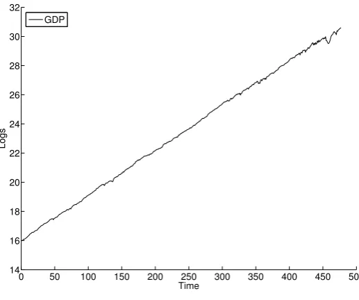
Figure 1: Log of GDP time series.
setup for which the model is empirically validated, i.e. it is able to replicate a wide spectrum of microeconomic and macroeconomic stylized facts. Next, we turn to “policy experiments”, by identifying sets of parameters (e.g. the interest rate, the credit multiplier, the tax rate) whose values capture different policies. Under the “policy experiment mode”, in Dosi et al. (2010), we studied the consequences of different “innovation regimes” — and related policies — and their interaction with (Keynesian) demand management. In this paper, we turn to experiments with different income distribution regimes and different fiscal and monetary policies, and we analyze their impact on a long list of indicators including output growth rates, output volatility, frequency of full employment and unemployment rates, likelihood of crises (defined as number of episodes with output growth rates lower than −3%).13 All results presented in the following sections refer to Montecarlo averages over 50 iterations of T=600 time steps each.14
The benchmark parameterization is reported in Appendix B.
4.1 Empirical Validation
Let us now consider the results of the empirical validation of the model. The macro and micro stylized facts robustly replicated by the model are the same statistical regularities produced by and discussed at much greater length in Dosi et al. (2010) plus a few other finance-related ones.15 So the model is able to generate macroeconomic series of output, consumption and aggregate
13Interestingly, many statistical regularities concerning the structure of the economy (e.g. firm size
distri-butions, fatness of firms growth rates, etc.) appear to hold across an ample parameter range, under positive technological progress, even when policies undergo the changes we study in the following.
14Preliminary tests show that results of the model are significantly robust to changes in the initial conditions
for the microeconomic variables of the model. In addition, they show that, for the majority of the statistics under study, Montecarlo distributions are sufficiently symmetric and unimodal. This justifies the use of across-run averages as meaningful indicators. All our results do not dramatically change if one increases Montecarlo sample sizes.
15See Stock and Watson (1999); Napoletano et al. (2006); Claessens et al. (2009) for the empirical properties
0 50 100 150 200 250 300 350 400 450 500 −0.4
−0.3 −0.2 −0.1 0 0.1 0.2 0.3
Time GDP
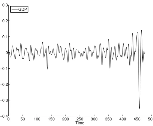
Figure 2: Bandpass filtered GDP series.
investment characterized by self-sustained growth patterns (see also Figure 1) and by persistent fluctuations (see also Figure 2 and Table 1). Moreover, aggregate investment is more volatile than GDP whereas consumption is less volatile. In addition, the model replicates the empirically observable co-movements between a large set of macro time series and GDP (net investment and consumption pro-cyclical coincident, inflation pro-cyclical and lagging, counter-cyclical mark-up rates, etc.).
At the same time, at the microeconomic level, the model matches a wide set of stylized facts concerning firm dynamics (including right-skewed distribution of firm sizes, fat-tailed dis-tributions of firm growth rates, wide and persistent productivity differences across firms, lumpy investment dynamics).
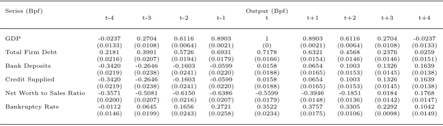
However, the credit-enhanced K+S model is also able to match the empirical evidence about the credit dynamics (see Claessens et al., 2009). As shown in Table 1, the model generates a highly pro-cyclical aggregate firm debt dynamics. Second, cross-correlation values shed light on the characteristics of the credit dynamics underneath the business cycles endogenously generated by the model, which has strong “Minskian” features (see e.g. Minsky, 1986). Indeed, bank deposits (equal to total firms’ net-worth) are counter-cyclical and lagging GDP. Supplied credit displays the same cyclical behavior and interestingly it is positively correlated with future values of GDP (cf. Table 1). This is in line with empirical evidence and it indicates that expansion in supplied credit anticipates future expansions in aggregate output.
Third, the net worth to sales ratio (proxying credit rating in the model) is counter-cyclical and lagging, whereas bankruptcy rates are pro-cyclical and coincident.
Series (Bpf) Output (Bpf)
t-4 t-3 t-2 t-1 t t+1 t+2 t+3 t+4
GDP -0.0237 0.2704 0.6116 0.8903 1 0.8903 0.6116 0.2704 -0.0237
(0.0133) (0.0108) (0.0064) (0.0021) (0) (0.0021) (0.0064) (0.0108) (0.0133) Total Firm Debt 0.2181 0.3991 0.5726 0.6931 0.7178 0.6321 0.4568 0.2376 0.0259
(0.0216) (0.0207) (0.0194) (0.0179) (0.0166) (0.0154) (0.0146) (0.0146) (0.0151) Bank Deposits -0.3420 -0.2646 -0.1603 -0.0599 0.0158 0.0654 0.1003 0.1326 0.1639
(0.0219) (0.0238) (0.0241) (0.0220) (0.0188) (0.0165) (0.0153) (0.0145) (0.0138) Credit Supplied -0.3420 -0.2646 -0.1603 -0.0599 0.0158 0.0654 0.1003 0.1326 0.1639
(0.0219) (0.0238) (0.0241) (0.0220) (0.0188) (0.0165) (0.0153) (0.0145) (0.0138) Net Worth to Sales Ratio -0.3571 -0.5081 -0.6150 -0.6386 -0.5599 -0.3946 -0.1851 0.0184 0.1768
(0.0200) (0.0207) (0.0216) (0.0207) (0.0179) (0.0148) (0.0136) (0.0142) (0.0147) Bankruptcy Rate -0.0112 0.0645 0.1656 0.2721 0.3522 0.3757 0.3305 0.2292 0.1042
(0.0146) (0.0199) (0.0243) (0.0258) (0.0234) (0.0175) (0.0106) (0.0098) (0.0149)
Table 1: Correlation structure for output and credit structure. Bpf: bandpass filtered (6,32,12) series. Monte-Carlo simulation standard errors in parentheses
.
100
10−3
10−2
10−1
100
Tail Distribution
Bad Debt
Simulation Data
Figure 3: Cross-sectional distribution of firms bad debt.
the premises for the incoming recessionary phase.
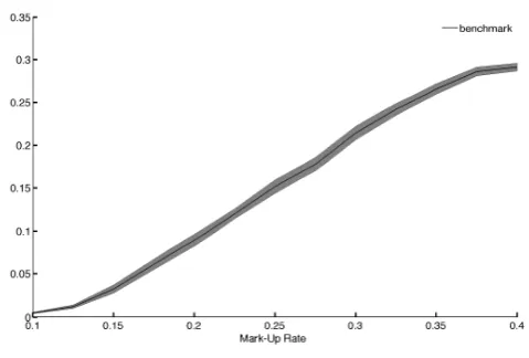
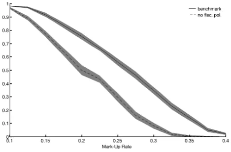
Figure 4: Frequency of full employment states the mark-up rates (95% confidence bands in gray).
Figure 5: Standard deviation of GDP growth rate and the mark-up rates (95% confidence bands in gray).
Figure 7: Unemployment rate and the mark-up rate (95% confidence bands in gray).
Figure 8: Average GDP growth rate and the mark-up rate (95% confidence bands in gray).
4.2 Income Distribution, Fiscal Policies, Growth and Business Cycles
The role played by mark-up rates in the dynamics of the model is twofold. On the one hand, the level of the mark-up determines the profits of the firms, and thus the level of internal resources available to finance production and investment expenditures. Higher mark-ups imply — ceteris paribus — higher profits and thus a lower dependence of firms on the external financing provided by banks. On the other hand, the mark-up regulates the distribution of income between profits and wages. Since aggregate consumption in the model is equal to total wages, higher mark-up rates result in a lower level of demand for final-good firms.
In light of these contrasting effects we explore the impact of different income distribution regimes on aggregate dynamics by varying the level of the mark-ups themselves. Figure 4 shows that the time the economy spends in full employment is inversely related to the mark-up rates. The more the functional distribution of income is biased towards profits, the less the economy spend time in full employment.
Figures 5, 6 and 7 reveal some further interesting features of such “non-Say” economies. First, the volatility of GDP growth (see Fig. 5) is positively related to the mark-up rate. Second, the incidence of crises (cf. Fig. 6) and relatively high unemployment states (cf. Fig. 7) are also higher.
The above patterns notwithstanding, the long-term average GDP growth rates (Figure 8) are only marginally (negatively) affected by the levels of mark-ups. Note however that the result is obtained in the “benchmark” scenario, which includes a positive level of fiscal redistributive policy (tax rates on profit to 40% redistributed as unemployment subsidies). If we repeat the same experiment with tax and subsidy rates both set to zero (see Figure 9), a pattern starkly emerges: if fiscal policies are absent, the adverse effects of the mark-up rate on the frequency of full employment states are strengthened.
The above findings generalize previous results from Dosi et al. (2010) on the role of fiscal policy in sustaining the long-term growth: the effectiveness of fiscal policy indeed increases with the mark-up. When the profit margin is very high, redistributive fiscal policies become a necessary condition for long-run growth. As in Dosi et al. (2010), redistributive policies act as a parachute when the economy experiences unemployment, by avoiding excessive falls in consumption demand due to the reduced incomes of unemployed workers. Moreover, investment expectations are linked to consumer demand in the model. Hence, more stable consumption demand profiles enhance the incentives to firms to invest in new capacity and in new machines. When the mark-up rate is low, the distribution of income is obviously in favor of wages. This implies a high propensity to consume and a high “investment accelerator”. As a consequence, the economy is most of the time in full employment. In contrast, when the profit margin is high, redistributive fiscal policies sustain an otherwise depressed consumer demand. This guarantees a higher long-run rate of growth.
Let us turn to a deeper investigation of the interactions between fiscal policies and income distribution regimes. More precisely, we define three scenarios according to the level of the initial mark-up rate (0.10; 0.20; 0.40) in the consumption-good sector, and we change simultaneously both the tax (t) (on profits only) and the unemployment-subsidy rates (wu) in the range between
under conditions on average of balanced-budget of government finances. Results are reported in Figures 10-15.
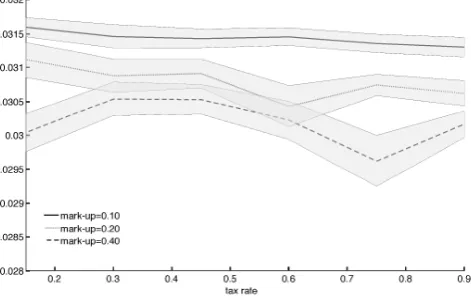
In all the three mark-up scenarios, the average growth rate is not significantly affected by changes in both the tax rates and the unemployment-subsidy (see Fig. 10). In contrast, the volatility of the economy and the incidence of crises are strongly reduced by higher unemploy-ment subsidy/tax rates (cf. Figs 11 and 14). Notice also that the effects of fiscal policies change according to the mark-up scenarios. Indeed, the capability of stronger redistributive policies to dampen business-cycle fluctuations increase when income distribution is more skewed toward profits.
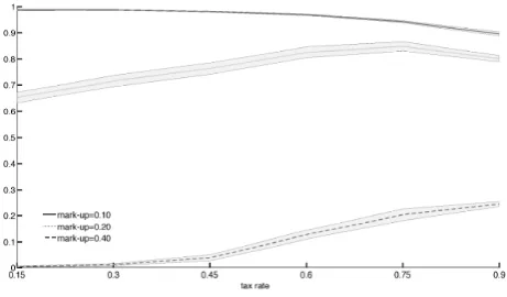
The same patterns emerge also on the labor market side. If income distribution strongly favor wages (i.e. ¯µ(0) = 0.10), the economy spends most of the time in full employment for every possible couples of tax and unemployment-subsidy (see Fig. 13). Of course this results in an average unemployment rate close to zero (cf. Fig. 12). For higher mark-up levels (i.e.
¯
µ(0) = 0.20; 0.40), higher doses of redistributive fiscal policies are required to stabilize the economy toward its full employment states.
Somewhat counterintuitively, the average bankruptcy rates (Fig. 15) arepositively influenced by higher levels of tax and unemployment subsidies. This occurs because stronger redistributive fiscal policies foster consumption demand and in turn firm investment, leading (extrapolatively adaptive) firms to build up what eventually will turn out to be excess productive capacity.
Overall, the results obtained in the three profit margin scenarios confirm the importance of the interactions between income distribution regimes and redistributive fiscal policies. In fact, expansionary policies happen to be even more needed under profit-biased income distributions: more or less the opposite to what EMU countries are currently trying to do!
Let us now study the effects of monetary policies.
4.3 Monetary Policy
Figure 10: Average GDP growth rate and the tax/unemployment-subsidy rates (95% confidence bands in gray).
Figure 11: Standard deviation of GDP growth rate and the tax/unemployment-subsidy rates (95% confidence bands in gray).
Figure 13: Frequency of full employment states and tax/unemployment-subsidy rates (95% confi-dence bands in gray).
Figure 14: Bankruptcy rate and tax/unemployment-subsidy rates (95% confidence bands in gray).
Interest Rates
As already mentioned, in this model we focus on a regime wherein inflation is on average zero, and we therefore rule out inflation targeting concerns. In addition, we make the extreme assumption that the Central Bank sets the initial level of the baseline interest rate and commits itself to keep it fixed throughout the simulation.
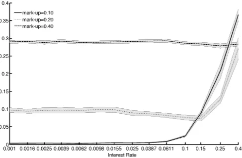
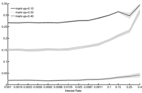
Figures 16 and 17 show the average GDP growth rate and its standard deviation as a function of the baseline interest rate r, for different mark-up levels. Both average growth and volatility are completely unaffected by changes in the interest rate in the high mark-up scenario (0.40).
In contrast, significant effects emerge in the “benchmark” and low mark-up scenarios (re-spectively 0.20 and 0.10; see Appendix B for benchmark parameterization). In these cases, the system displays two phases (i.e. two regimes). The interest rate does not change average growth and volatility up to a threshold above which average growth start decreasing and volatility in-creasing with the interest rate (see Figures 16 and 17). In addition, the threshold above which the interest rate affects growth and volatility decreases with the mark-up level.
The patterns displayed by other real variables in the model are similar to the ones just described. Interest rates have no effects on the average unemployment rate (Figure 19) and on the likelihood of crises (Figure 18), if the mark-up is very high (0.40). At lower levels (0.20, 0.10), interest rates affect unemployment and the likelihood of crises above a given threshold value, with both unemployment and the probability of crises steadily increasing with interest rates.
The general picture is that, when mark-up rates are sufficiently low, changes in interest rates may affect real dynamics in a significant way. In particular high interest rates bring the economy on a low growth trajectory, characterized by wide fluctuations in output and high average unemployment rates. And this outcome is strongly correlated to the fall in the frequency of periods the economy spends in full employment (see Figure 20).
Figure 16: Average GDP growth and the interest rate (95% confidence bands in gray).
Figure 17: Standard deviation of GDP growth rate and the interest rate (95% confidence bands in gray).
Figure 19: Unemployment rate and the interest rate (95% confidence bands in gray).
Figure 20: Frequency of full employment states and the interest rate (95% confidence bands in gray).
Credit Multipliers
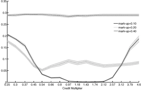
How do the above results change when one varies the maximum credit available in the economy? Figure 22 shows average GDP growth as a function of the credit multiplier in turn determined by reserve requirements imposed by the Central Bank in different mark-up scenarios.16 Similarly to
the interest rate experiment, the sensitivity of real variables to changes in the credit multiplier decreases with mark-up rates. It is null in the case of high mark-ups (0.40), and it is the highest for a level of mark-up equal to 0.10. Let us then focus on this latter scenario. Figure 22 shows that the relation between average GDP growth and the credit multiplier is quite asymmetric. Namely, credit “contractions” negatively affect growth. In contrast, expanding total credit above a certain threshold does not lead to significant improvements in growth performance. Also average volatility is significantly affected by changes in the credit multiplier (cf. Figure 23) and, interestingly, the relation is U-shaped. Volatility is the highest for low and high values of the ratio, while it is minimized for intermediate values. This is due to the effects that this instrument has on the credit supply. Lower levels of the multiplier reduce the availability of loans, forcing firms to rely more on their highly volatile net profits. At the opposite end, much higher credit multipliers allow firms to explosively finance production and investment, eventually leading to overproduction and overinvestment episodes.
This U-shaped pattern is even more evident in the analysis of the likelihood of crises (see Fig. 24). Under intermediate values, such a likelihood is strikingly low.
These results uncover another interesting property of the model: raising too much the credit multiplier brings only small contributions to the long-run growth of the economy. At the same time it leads to wider fluctuations and to a higher incidence of crises. In contrast, decreasing too much the multiplier increases both volatility and crises, and also reduces the growth prospects of the economy.
The relationship between credit multiplier and business cycle fluctuations also affects the unemployment rate. Increases in the credit multiplier yield to a dramatic fall of the unemploy-ment rate up to a threshold above which the higher volatility of the economy is reflected also in increasing levels of unemployment (see Figs. 25 and 26).
Monetary policy effects: a discussion
Let us now summarize as well as provide some general interpretations of the above findings. First, the results show deep interactions between monetary policies and patterns of income distribution between wages and profits. In particular the lack of sensitivity to changes in monetary policy variables at high mark-up rates, indicates the possible emergence of a sort of liquidity traps.17
Increasing mark-ups raises the availability of internal funds to firms. At the same time, lower wage shares imply lower aggregate consumption propensity.18 Via demand expectations, this leads to a lower propensity to invest into the expansion of the productive capacity. When
mark-16The following discussion focuses on the effects of credit multipliers. However, results do not change if one
changes credit ceilings to single firms instead of the maximum credit supply available in the economy.
17This type of liquidity trap is of course different from the standard Keynesian one. There agents prefer to
keep their funds as money rather than investing them into bonds. Here, instead firms prefer to keep their funds as money instead of investing into activities such as production and investment.
18In our model, to repeat, we make the extreme assumption that all wages are consumed and all profits are
Figure 22: Average GDP growth and the credit multiplier rate (95% confidence bands in gray).
Figure 23: Standard deviation of GDP growth rate and the credit multiplier rate (95% confidence bands in gray).
Figure 25: Unemployment rate and the credit multiplier rate (95% confidence bands in gray).
ups are too high, the second force becomes dominant, and therefore firms have plenty of idle funds which are kept as money (more precisely deposits), rather then being invested. In this case, monetary policies can do little to influence the economy, as the low propensity to invest implies also low incentives to raise debt. Second, even when mark-ups are low (and thus the sensitivity to monetary policy interventions is in principle high) there are regions of monetary policy ineffectiveness: our results indicate the existence of threshold values below which changes in interest rate or in the credit multiplier have small or no effect on real variables.
Furthermore, the different role played by interest rate vs. credit quantity instruments (credit multipliers) can be explained on the grounds of the different transmission mechanisms through which these instruments operate.
Consider interest rates. First, the level of interest rate affects the real sector through a “balance sheet channel”. By impacting on firms’ costs, the levels of interest rates determine firms’ net cash flows available to finance production and investment plans and symmetrically the requirements of external financing. Second, by determining bank’s and firms’ profits, interest rates directly affect the amount of funds redistributed from the real sector to the banking sector. Bank’s profits are added to bank reserves, and therefore are not reinvested into credit to firms. It is straightforward that high interest rates imply — ceteris paribus — lower net profits of firms and therefore — via the “bank lending channel” — a lower amount of resources available to finance production and investment expenditures.
Credit multipliers influence too the total level of credit available in the economy. However, by not impacting on firms’ costs they do not alter the dynamics of internal funds and the demand for credit of individual firm. This explains also why credit multipliers basically affect the growth of the economy only on the “downside”, when the squeeze on credit availability induces a sort of systemic rationing of the economy.
5
Concluding Remarks
In this paper we have explored the interactions between the financial and real sides of an evo-lutionary agent-based economy under different mixes of fiscal and monetary policies. After showing the ability of the model to reproduce the main stylized facts concerning credit dynam-ics at the micro and macro levels, we analyzed the effects of fiscal and monetary policies under different conditions characterizing the distribution of income between wages and profits. Our results emphasize the high interdependence between macro policies and the patterns of income distribution. In presence of a high profit bias, redistributive fiscal policies are able to dampen business cycle fluctuations and to keep the economy close to full employment. In line with the result shown in Dosi et al. (2010) we find that some fiscal policies are in any case necessary to keep the system away from a stagnant long-term trajectory, even in presence of abundant “Schumpeterian” opportunities of innovation.
The results of our experiment strongly support the old-fashion Keynesian view of economic policies with their relative emphasis on fiscal ones both as countercyclical instruments and as necessary conditions to keep the economy on a “virtuous” high growth path. Needless to say, if there is some truth in our conclusions they run exactly counter the current European recipes: the recent fiscal austerity programs pursued by EMU countries are likely to worsen the state of the economy, further lowering the rate of growth, and increasing the instability of European economies.
The present work could be extended in at least three directions. First, in this model we deliberately focused on a regime wherein average inflation is zero and where the Central Bank interest rate is fixed throughout the experiments. This takes away the effects of further dis-tributive changes induced by different inflation rates. In addition, it allows one to study more neatly the dynamic consequences on output and unemployment of persistent interest rate poli-cies. However, one could easily extend the analysis to a framework in which average inflation can be positive and where the Central Bank adjusts interest rates and credit conditions in the light of some output and inflation targeting (the famous Taylor Rule being one of the possible strategies).
Second, one could extend the present framework to one wherein heterogeneous banks are present. This would allow one to study the macroeconomic effects of banking crises and the consequences on output and public finances of different bail-out schemes.
Finally, here we considered a regime where workers fully consume their wage. However, one could move to a framework which allows for the possibility of household savings and indebted-ness. The latter played an important role in the recent crisis. Indeed, we conjecture, they are likely to strengthen the credit dynamics discussed in the previous sections.
Acknowledgements
References
Akerlof, G. A., 2002. Behavioral Macroeconomics and Macroeconomic Behavior. American Economic Review. 92, 411–433.
Ashraf, Q., Gershman, B. and Howitt, P., 2011. Banks, Market Organization, and Macroeconomic Performance: An Agent-Based Computational Analysis. Working Paper 17102. NBER.
Atkinson, A. B. and Piketty, T. (eds), 2010. Top Incomes: A Global Perspective. Oxford University Press.
Bartelsman, E. and Doms, M., 2000. Understanding Productivity: Lessons from Longitudinal Microdata. Journal of Economic Literature. 38, 569–94.
Bernanke, B., Gertler, M. and Gilchrist, S., 1999. The Financial Accelerator in a Quantitative Business Cycle Framework. InHandbook of Macroeconomics, J. Taylor and M. Woodford (eds). Elsevier Science: Amsterdam. Bernanke, B. S. and Blinder, A. S., 1988. Credit, Money, and Aggregate Demand. American Economic Review.
782, 435–39.
Bernanke, B. S. and Blinder, A. S., 1992. The Federal Funds Rate and the Channels of Monetary Transmission. American Economic Review. 824, 901–21.
Black, L. and Rosen, R., 2011. The effect of monetary policy on the availability of credit: How the credit channel works. Working Paper 2007-13. FRB of Chicago.
Charpe, M., Flaschel, P., Proano, C. and Semmler, W., 2009. Overconsumption, credit rationing and bailout monetary policy: A Minskyan perspective. European Journal of Economics and Economic Policies. 62, 247– 270.
Chiarella, C., Flaschel, P. and Semmler, W., 1999. The Macrodynamics of Debt Deflation. SCEPA Working Papers 1999-04. Schwartz Center for Economic Policy Analysis (SCEPA), The New School.
Christiano, L. G., Eichenbaum, M. and Evans, C. L., 2005. Nominal Rigidities and the Dynamic Effects of a Shock to Monetary Policy. Journal of Political Economy. 113, 1–45.
Ciarli, T., Lorentz, A., Savona, M. and Valente, M., 2010. The Effect of Consumption and Production Structure on Growth and Distribution. A Micro to Macro Model. Metroeconomica. 611, 180–218.
Ciccarelli, M., Maddaloni, A. and Peydr´o, J.-L., 2010. Trusting the Bankers: A New Look at the Credit Channel of Monetary Policy. Working Paper Series 1228. European Central Bank.
Cincotti, S., Raberto, M. and Teglio, A., 2010. Credit Money and Macroeconomic Instability in the Agent-based Model and Simulator Eurace. Economics: The Open-Access, Open-Assessment E-Journal. 42010-26.
Claessens, S., Kose, M. and Terrones, M., 2009. What happens during recessions, crunches and busts?. Economic Policy. 2460, 653–700.
Dawid, H., Fagiolo, G. and Roventini, A., 2012. Macroeconomic Policy in Agent-Based and DSGE Models. Working paper. Laboratory of Economics and Management (LEM).
Dawid, H., Gemkow, S., Harting, P., Kabus, K., Neugart, M. and Wersching, K., 2008. Skills, Innovation, and Growth: An Agent-Based Policy Analysis. Journal of Economics and Statistics. forthcoming.
Dawid, H., Gemkow, S., van der Hoog, S. and Neugart, M., 2011. The Eurace@Unibi Model: An Agent-Based Macroeconomic Model for Economic Policy Analysis. Working paper. Universit¨at Bielefeld.
Del Boca, A., Galeotti, M., Himmelberg, C. P. and Rota, P., 2008. Investment and Time to Plan and Build: A Comparison of Structures vs. Equipment in A Panel of Italian Firms. Journal of the European Economic Association. 6, 864–889.
Delli Gatti, D., Desiderio, S., Gaffeo, E., Cirillo, P. and Gallegati, M., 2011. Macroeconomics from the Bottom-up. Springer: Milan.
Delli Gatti, D., Gallegati, M., Greenwald, B., Russo, A. and Stiglitz, J., 2010. The Financial Accelerator in an Evolving Credit Network. Journal of Economic Dynamics & Control. 34, 1627–1650.
Di Guilmi, C., Gallegati, M. and Ormerod, P., 2004. Scaling invariant distributions of firms exit in OECD countries. Physica A: Statistical Mechanics and its Applications. 3341, 267–273.
Doms, M. and Dunne, T., 1998. Capital Adjustment Patterns in Manufacturing Plants. Review Economic Dy-namics. 1, 409–29.
Dosi, G., 2007. Statistical Regularities in the Evolution of Industries. A Guide through some Evidence and Challenges for the Theory. InPerspectives on Innovation, F. Malerba and S. Brusoni (eds). Cambridge MA, Cambridge University Press.
Dosi, G., 2011. Economic Coordination and Dynamics: Some Elements of an Alternative “Evolutionary” Paradigm. Technical report. Institute for New Economic Thinking.
Dosi, G., Fagiolo, G. and Roventini, A., 2006. An Evolutionary Model of Endogenous Business Cycles. Compu-tational Economics. 27, 3–34.
Dosi, G., Fagiolo, G. and Roventini, A., 2010. Schumpeter Meeting Keynes: A Policy-Friendly Model of Endoge-nous Growth and Business Cycles. Journal of Economic Dynamics & Control. 34, 1748–1767.
Eisner, R., 1972. Components of Capital Expenditures: Replacement and Modernization versus Expansion. The Review of Economics and Statistics. 54, 297–305.
Fabiani, S., Druant, M., Hernando, I., Kwapil, C., Landau, B., Loupias, C., Martins, F., Math¨a, T., Sabbatini, R., Stahl, H. and Stokman, A., 2006. What Firms’ Surveys Tell Us about Price-Setting Behavior in the Euro Area. International Journal of Central Banking. 2, 3–47.
Fazzari, S., Ferri, P. and Greenberg, E., 2008. Cash Flow, Investment, and Keynes–Minsky cycles. Journal of Economic Behavior & Organization. 653, 555–572.
Fazzari, S. M., Hubbard, G. R. and Petersen, B. C., 1988. Financing Constraints and Corporate Investment. Brookings Papers on Economic Activity. 1, 141–95.
Feldstein, M. and Foot, D., 1971. The Other Half of Gross Investment: Replacement and Modernization Expen-ditures. The Review of Economics and Statistics. 53, 49–58.
Fisher, I., 1933. The Debt-Deflation Theory of Great Depressions. Econometrica. 1, 337–357.
Fitoussi, J. and Saraceno, F., 2010. Inequality and Macroeconomic Performance. Document de Travail 2010-13. OFCE.
Fujiwara, Y., 2004. Zipf law in firms bankruptcy. Physica A: Statistical and Theoretical Physics. 3371-2, 219–230.
Gai, P., Haldane, A. and Kapadia, S., 2011. Complexity, Concentration and Contagion. Journal of Economic Dynamics & Control. 58, 453–470.
Gertler, M., 1988. Financial Structure and Aggregate Economic Activity: An Overview. Journal of Money, Credit and Banking. 203, 559–88.
Gertler, M. and Gilchrist, S., 1994. Monetary Policy, Business Cycles, and the Behavior of Small Manufacturing Firms. The Quarterly Journal of Economics. 1092, 309–40.
Gertler, M. and Kiyotaki, N., 2010. Financial Intermediation and Credit Policy in Business Cycle Analysis. In
Handbook of Monetary Economics, B. M. Friedman and M. Woodford (eds). North Holland, Amsterdam. Goolsbee, A., 1998. The Business Cycle, Financial Performance, and the Retirement of Capital Goods. Working
Paper 6392. NBER.
Greenwald, B. and Stiglitz, J., 1993. Financial Market Imperfections and Business Cycles. Quarterly Journal of Economics. 108, 77–114.
Gurley, J. and Shaw, E., 1955. Financial aspects of economic development. American Economic Review. 45, 515– 538.
Hubbard, G. R., 1998. Capital-Market Imperfections and Investment. Journal of Economic Literature. 36, 193– 225.
Kashyap, A. K. and Stein, J. C., 2000. What Do a Million Observations on Banks Say about the Transmission of Monetary Policy?. American Economic Review. 903, 407–428.
Kashyap, A. K., Stein, J. C. and Wilcox, D. W., 1993. Monetary Policy and Credit Conditions: Evidence from the Composition of External Finance. American Economic Review. 831, 78–98.
Keen, S., 1995. Finance and Economic Breakdown: Modeling Minsky’s ”Financial Instability Hypothesis”. Journal of Post Keynesian Economics. 174, 607–635.
Keynes, J. M., 1936. The General Theory of Employment, Interest, and Money. New York, Prometheus Books.
Kindleberger, C., 1978. Manias, Panics, and Crashes. New York, Basic Books.
Kirman, A. P., 1992. Whom or What Does the Representative Individual Represent?. Journal of Economic Perspectives. 6, 117–136.
Kirman, A. P., 2010. The Economic Crisis is a Crisis for Economic Theory. CESifo Economic Studies. 56, 498–535.
Kiyotaki, N. and Moore, J., 1997. Credit Cycles. Journal of Political Economy. 1052, 211–48.
Krugman, P. (2011) Mr. Keynes and the “Moderns”. prepared for the Cambridge conference commemorating the 75th anniversary of the publication of The General Theory of Employment, Interest, and Money.
Kumhof, M. and Ranciere, R., 2010. Inequality, Leverage and Crisis. Working Paper WP/10/268. IMF.
Leary, M., 2009. Bank Loan Supply, Lender Choice, and Corporate Capital Structure. The Journal of Finance. 643, 1143–1185.
LeBaron, B. and Tesfatsion, L., 2008. Modeling Macroeconomies as Open-Ended Dynamic Systems of Interacting Agents. American Economic Review. 98, 246–250.
Lown, C. and Morgan, D., 2006. The Credit Cycle and the Business Cycle: New Findings Using the Loan Officer Opinion Survey. Journal of Money, Credit, and Banking. 386, 1575–1597.
Minsky, H., 1975. John Maynard Keynes. London: Macmillan. pp. 1106–108.
Minsky, H., 1977. The Financial Instability Hypothesis: an Interpretation of Keynes and an Alternative to Standard Theory. Challenge. 201, 20–27.
Minsky, H., 1982. Can It Happen Again?. M.E. Sharpe. New York.
Minsky, H., 1986. Stabilizing an Unstable Economy. Yale University Press (New Haven).
Mishkin, F., 1995. Symposium on the Monetary Transmission Mechanism. The Journal of Economic Perspectives. 94, 3–10.
Modigliani, F. and Miller, M., 1958. The Cost of Capital, Corporation Finance and the Theory of Investment. American Economic Review. 48, 261–97.
Napoletano, M., Roventini, A. and Sapio, S., 2006. Are Business Cycles All Alike? A Bandpass Filter Analysis of the Italian and US Cycles. Rivista Italiana degli Economisti. 1, 87–118.
Nelson, R. R. and Winter, S. G., 1982. An Evolutionary Theory of Economic Change. Cambridge, The Belknap Press of Harvard University Press.
Palley, T., 1994. Debt, Aggregate Demand, and the Business Cycle: an Analysis in the Spirit of Kaldor and Minsky. Journal of Post Keynesian Economics. 163, 371–390.
Rosser, B. J., 2011. Complex Evolutionary Dynamics in Urban-Regional and Ecologic-Economic Systems: From Catastrophe to Chaos and Beyond. Springer: New York.
Russo, A., Catalano, M., Gallegati, M., Gaffeo, E. and Napoletano, M., 2007. Industrial Dynamics, Fiscal Policy and R&D: Evidence from a Computational Experiment. Journal of Economic Behavior and Organization. 64, 426–447.
Saviotti, P. and Pyka, A., 2008. Product Variety, Competition and Economic Growth. Journal of Evolutionary Economics. 18, 323–347.
Smets, F. and Wouters, R., 2007. Shocks and Frictions in US Business Cycles: A Bayesian DSGE Approach. American Economic Review. 97, 586–606.
Solow, R. M., 2008. The State of Macroeconomics. Journal of Economic Perspectives. 22, 243–246.
Stiglitz, J., 2011. Rethinking Macroeconomics: What Failed, and How to Repair It. Journal of the European Economic Association. 9, 591–645.
Stiglitz, J. and Weiss, A., 1992. Credit Rationing in Markets with Imperfect Information. American Economic Review. 71, 393–410.
Stock, J. and Watson, M., 1999. Business Cycle Fluctuations inU.S.Macroeconomic Time Series. InHandbook of Macroeconomics, J. Taylor and M. Woodford (eds). Amsterdam, Elsevier Science.
Taylor, L. and O’Connell, S., 1985. A Minsky crisis. The Quarterly Journal of Economics. 100, 871–885.
Tesfatsion, L. and Judd, K. (eds), 2006. Handbook of Computational Economics II: Agent-Based Computational Economics. North Holland, Amsterdam.
Verspagen, B., 2002. Evolutionary Macroeconomics: A Synthesis between Neo-Schumpeterian and Post-Keynesian Lines of Thought. The Electronic Journal of Evolutionary Modeling and Economic Dynamics. 1007.
A
Analytical Description of the Model
In this appendix we present the full formal structure of the real side of the model discussed in Section 3. We start with the equations characterizing search processes and the determination of production and prices in the capital-good sector. Next we turn to present the equations related to the determination of production, investment, prices and profits in the consumption-good sector.
A.1 The Capital-Good Industry
In the capital-good sector there areF1firms denoted by the subscripti. The technology of a capital-good firms is
defined by the vector (Aτi, B τ
i), where the former coefficient is the productivity of the manufactured machine-tool
in the consumption-good industry, the latter coefficient is the efficiency of the production technique employed by the firm, and the positive integerτ denotes the current technology vintage. Given the monetary wagew(t), the unit cost of production of capital-good firms is:
ci(t) =
The unit labor cost of production entailed by a machine in the consumption-good sector is:
c(Aτi, t) =
w(t)
Aτ i
.
Capital-good firms invest in R&D a fraction of their past sales (Si):
RDi(t) =νSi(t−1), (12)
with 0< ν <1. R&D expenditures are used to hire researchers paying the market wagew(t). Firms split their R&D efforts between innovation (IN) and imitation (IM) according to the parameterξ∈[0,1]:
INi(t) =ξRDi(t)
IMi(t) = (1−ξ)RDi(t).
We model innovation as a two steps process. The first step determines whether a firm successfully innovates or not through a draw from a Bernoulli distribution, whose parameterθiin(t) is given by:
θiin(t) = 1−e
the interval [−1,0] andx1 to [0,1]19. Imitation follows a two steps procedure as well. The set of successfully
imitating firms is formed sampling from a Bernoulli(θimi (t)):
θimi (t) = 1−e
−ζ2IMi(t), (14)
with 0< ζ261. Firms accessing the second stage are able to copy the technology of one competitor (Aimi , Biim).
We assume that firms are more likely to imitate competitors with similar technologies. For that, we use an Eu-clidean metrics to compute the technological distance between every pair of firms to weight imitation probabilities.
19We choose the Beta distribution because of its flexibility, able in particular to capture, according to the