Fundamentals of Digital Image Processing

Fundamentals

of Digital

Image Processing

ANIL K. JAIN

University of California, Davis

II

3

Image Perception

3.1 INTRODUCTION

In presenting the output of an imaging system to a human observer, it is essential to consider how it is transformed into information by the viewer. Understanding of the visual perception process is important for developing measures of image fidelity, which aid in the design and evaluation of image processing algorithms and imaging systems. Visual image data itself represents spatial distribution of physical quan­ tities such as luminance and spatial frequencies of an object. The perceived infor­ mation may be represented by attributes such as brightness, color, and edges. Our primary goal here is to study how the perceptual information may be represented quantitatively.

3.2 LIGHT, LUMINANCE, BRIGHTNESS, AND CONTRAST

Light is the electromagnetic radiation that stimulates our visual response. It is expressed as a spectral energy distribution L (X. ), where X. is the wavelength that lies in the visible region, 350 nm to 780 nm, of the electromagnetic spectrum. Light received from an object can be written as

/(X.) = p(X.)L(X.) (3.1)

where p(ll.) represents the reflectivity or transmissivity of the object and L (X.) is the incident energy distribution. The illumination range over which the visual system can operate is roughly 1 to 1010, or 10 orders of magnitude.

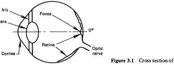
The retina of the human eye (Fig. 3 . 1) contains two types of photoreceptors called rods and cones. The rods, about 100 million in number, are relatively long and thin. They provide scotopic vision, which is the visual response at the lower several orders of magnitude of illumination. The cones, many fewer in number

�

:;-The eye

Iris

Lens

Optic nerve

Figure 3.1 Cross section of the eye.

(about 6.5 million), are shorter and thicker and are less sensitive than the rods. They provide photopic vision, the visual response at the higher 5 to 6 orders of magnitude of illumination (for instance, in a well-lighted room or bright sunlight). In the intermediate region of illumination, both rods and cones are active and provide

mesopic vision. We are primarily concerned with the photopic vision, since elec­ tronic image displays are well lighted.

The cones are also responsible for color vision. They are densely packed in the center of the retina (called fovea) at a density of about 120 cones per degree of arc subtended in the field of vision. This corresponds to a spacing of about 0.5 min of arc, or 2 µm. The density of cones falls off rapidly outside a circle of 1° radius from the fovea. The pupil of the eye acts as an aperture. In bright light it is about 2 mm in diameter and acts as a low-pass filter (for green light) with a passband of about 60 cycles per degree.

The cones are laterally connected by horizontal cells and have a forward connection with bipolar cells. The bipolar cells are connected to ganglion cells, which join to form the optic nerve that provides communication to the central nervous system.

The luminance or intensity of a spatially distributed object with light distribu­ tion I(x, y, X.) is defined as

f(x, y) =

r

I(x, y, X.)V(X.) dX.

0 (3.2)

where V(X.) is called the relative luminous efficiency function of the visual system. For the human eye, V(X.) is a bell-shaped curve (Fig. 3.2) whose characteristics

1 .0

0.8

0.6

0.4

0.2

0

380 460 540 620 700 A(nm)

780 _{Figure 3.2 Typical relative luminous ef­}

depend on whether it is scotopic or photopic vision. The luminance of an object is independent of the luminances of the surrounding objects. The brightness (also called apparent brightness) of an object is the perceived luminance and depends on the luminance of the surround. Two objects with different surroundings could have

identical luminances but different brightnesses. The following visual phenomena exemplify the differences between luminance and brightness.

Simultaneous Contrast

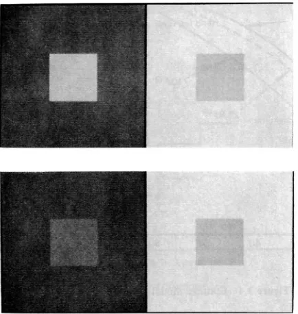
In Fig. 3.3a, the two smaller squares in the middle have equal luminance values, but the one on the left appears brighter. On the other hand in Fig. 3.3b, the two squares appear about equal in brightness although their luminances are quite different. The reason is that our perception is sensitive to luminance contrast rather than the absolute luminance values themselves.

According to Weber's law [2, 3] , if the luminance fa of an object is just noticeably different from the luminance ls of its surround, then their ratio is

Ifs -fa _{I = constant (3.3)}

fa

Writingf0 = f, ls = f + Llf where Llf is small for just noticeably different luminances, (3.3) can be written as

J

= d(logf) = lie (constant) (3.4) The value of the constant has been found to be 0.02, which means that at least 50 levels are needed for the contrast on a scale of 0 to 1 . Equation (3.4) says

Sec. 3.2

Figure 3.3 Simultaneous contrast: (a) small squares in the middle have equal luminances but do not appear equally bright;

(b) small squares in the middle appear almost equally bright, but their lumi­ nances are different.

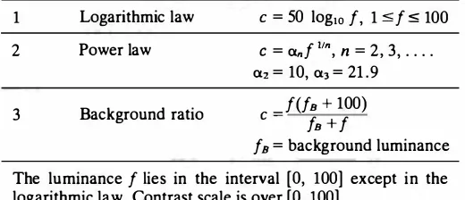
TABLE 3.1 Luminance to Contrast Models

1 Logarithmic law

2 Power law

3 Background ratio

c = 50 log10 f, 1 :s;f:s; 100

C = anf 11n, n = 2, 3, . . . .

a2 = 10, a3 = 21 .9 f(fB + 100)

C =

fB + f

f B = background luminance The luminance f lies in the interval [O, 100] except in the logarithmic law. Contrast scale is over [O, 100].

equal increments in the log of the luminance should be perceived to be equally different, i.e . , d(logf ) is proportional to de, the change in contrast. Accordingly, the quantity

(3.5)

where a1 , a2 are constants, is called the contrast. There are other models of contrast [see Table 3.1 and Fig. 3.4], one of which is the root law

C =

Jlln (3.6)

The choice of n = 3 has been preferred over the logarithmic law in an image coding study [7]. However, the logarithmic law remains the most widely used choice.

1 00

80

(.J 60

tf

� i: 2 1 .9f113

0 tJ ₄₀

20

0 20 40 60 80 1 00

Luminance, f

Mach Bands

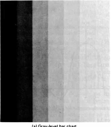
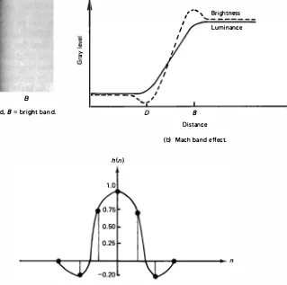
The spatial interaction of luminances from an object and its surround creates a phenomenon called the Mach band effect. This effect shows that brightness is not a monotonic function of luminance. Consider the gray level bar chart of Fig. 3.Sa, where each bar has constant luminance. But the apparent brightness is not uniform along the width of the bar. Transitions at each bar appear brighter on the right side and darker on the left side. The dashed line in Fig. 3.Sb represents the perceived brightness. The overshoots and undershoots illustrate the Mach band effect. Mach bands are also visible in Fig. 3.6a, which exhibits a dark and a bright line (marked D and B ) near the transition regions of a smooth-intensity ramp. Measurement of the

(a) Gray-level bar chart.

Luminance

r�-- - - Brightness

�---....: r�---J ...---, _{- - - -�} - - - --�

-- - - -�

D istance

(b) Luminance versus brightness. Figure J.5 Mach band effect.

D B - - - ....

(a) D = dark band, 8 = bright band. _D

h(n)

1 .0

I I l

/-', Brightness ... _ _ _ _ _ _ _

I

I Luminance

8

Distance

(b) Mach band effect.

(c) Nature of the visual system impulse response.

Figure 3.6 Mach bands.

Mach band effect can be used to estimate the impulse response of the visual system (see Problem 3.5).

Figure 3.6c shows the nature of this impulse response. The negative lobes manifest a visual phenomenon known as lateral inhibition. The impulse response values represent the relative spatial weighting (of the contrast) by the receptors, rods and cones. The negative lobes indicate that the neural (postretinal) signal at a given location has been inhibited by some of the laterally located receptors.

3.3 MTF OF THE VISUAL SYSTEM

Cii 50 '.!:!.

� 40 ·:;

·;:; ·;;;

c: ₃₀

ill �

"' E 20

c: ₀ (.) _{1 0}

0 0.5 5 1 0

(a) _{Spatial frequency, cycles/degree}

(b)

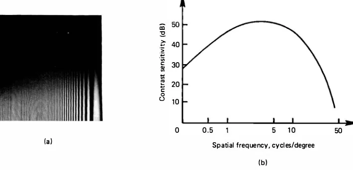
Figure 3.7 MTF of the human visual system. (a) Contrast versus spatial frequency sinusoidal grating; (b) typical MTF plot.

50

various frequencies. The curve representing these thresholds is also the MTF, and it varies with the viewer as well as the viewing angle. Its typical shape is of the form shown in Fig. 3.7b. The curve actually observed from Fig. 3.7a is your own MTF (distorted by the printing process). The shape of the curve is similar to a band-pass filter and suggests that the human visual system is most sensitive to midfrequencies and least sensitive to high frequencies. The frequency at which the peak occurs varies with the viewer and generally lies between 3 and 10 cycles/degree. In practice, the contrast sensitivity also depends on the orientation of the grating, being maximum for horizontal and vertical gratings. However, the angular sensitivity variations are within 3 dB (maximum deviation is at 45°) and, to a first approxi­ mation, the MTF can be considered to be isotropic and the phase effects can be ignored. A curve fitting procedure [6] has yielded a formula for the frequency response of the visual system as

p = Y � i + _{� �} cycles/degree (3.7) where A, a, 13, and p0 are constants. For a = 0 and 13

=

1 , p0 is the frequency at

which the peak occurs. For example, in an image coding application [6], the values A = 2.6, a = 0.0192, p0 = (0. 1 14t1 = 8.772, and 13 = 1 . 1 have been found useful.

The peak frequency is 8 cycles/degree and the peak value is normalized to unity.

3.4 THE VISIBILITY FUNCTION

In many image processing systems-for instance, in image coding-the output image u· (m, n) contains additive noise q (m, n ), which depends on e (m, n ), a func­ tion of the input image u(m, n) [see Fig. 3.8]. The sequence e(m, n) is sometimes called the masking function. A masking function is an image feature that is to be

u(m, n) + u"(m, n)

---""i + _ ____,� +

q(m, n)

Noise

source Figure 3.8 Visibility function noise

source model. The filter impulse response

h (m, n) determines the masking func­ tion. Noise source output depends on the masking function amplitude

lei-observed or processed in the given application. For example, e(m, n) = u (m, n) in PCM transmission of images. Other examples are as follows:

1.

e(m, n)

=

u(m, n) - u (m - 1, n)

2. e(m, n) = u(m, n) - a1 u(m - 1, n) - a2u(m, n - l) + a3u(m - 1, n - l)

3. e(m, n) = u(m, n) - u[u(m - l , n) + u(m + l , n)

+ _{u (m, n - l)} + _{u(m, n} + _1)]

The visibility function measures the subjective visibility in a scene containing this masking function dependent noise q(m, n). It is measured as follows. For a suitably small At and a fixed interval [x, x + At], add white noise of power P, to all those pixels in the original image where masking function magnitude le I lies in this interval. Then obtain another image by adding white noise of power Pw to all the pixels such that the two images are subjectively equivalent based on a subjective scale rating, such as the one shown in Table 3.3. Then the visibility function v(x) is defined as [4]

where

v(x) = -dV(x) dx

V(x)

=

Pw

P,

(3.8)

The visibility function therefore represents the subjective visibility in a scene of unit masking noise. This function varies with the scene. It is useful in defining a quantita­

tive criterion for subjective evaluation of errors in an image (see Section 3.6).

3.5 MONOCHROME VISION MODELS

Light

L (x, y, ;\)

Eye optics

H,(�,. �2) J (x, y, ;\)

V(;>..) Luminance -f(x, y) Spectral response V(;\)

� - - - -1

I _I

I

I Brightne Lum inance Cone Contrast Lateral SS

-response

-f(x, y) g( . ) c(x, y)

I

I

inhibition

H(�1. bl

I

-I

I b(x, y)

L - - - �

c

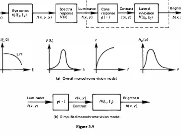
(a) Overall monochrome vision model.

c(x, y) Brightness

g( . ) _{H(�, .} t2)

-Contrast

-b(x, y)

(b) Simplified monochrome vision model.

Figure 3.9

g ( · ), yields the contrast c (x, y ). The lateral inhibition phenomenon is represented by a spatially invariant, isotropic, linear system whose frequency response is H(�1 , �2). Its output is the neural signal, which represents the apparent brightness

b (x, y). For an optically well-corrected eye, the low-pass filter has a much slower drop-off with increasing frequency than that of the lateral inhibition mechanism. Thus the optical effects of the eye could be ignored, and the simpler model showing the transformation between the luminance and the brightness suffices.

Results from experiments using sinusoidal gratings indicate that spatial fre­ quency components, separated by about an octave, can be detected independently by observers. Thus, it has been proposed [7] that the visual system contains a number of independent spatial channels, each tuned to a different spatial frequency and orientation angle. This yields a refined model, which is useful in the analysis and evaluation of image processing systems that are far from the optimum and introduce large levels of distortions. For near-optimum systems, where the output image is only slightly degraded, the simplified model in Fig. 3.9 is adequate and is the one with which we shall mostly be concerned.

3.6 IMAGE FIDELITY CRITERIA

Image fidelity criteria are useful for measuring image quality and for rating the performance of a processing technique or a vision system. There are two types of criteria that are used for evaluation of image quality, subjective and quantitative. The subjective criteria use rating scales such as goodness scales and impairment

TABLE 3.2 Image Goodness Scales Overall goodness scale Excellent Good Fair Poor Unsatisfactory (5) (4) (3) (2) (1)

Group goodness scale Best

Well above average Slightly above average Average

Slightly below average Well below average Worst (7) (6) (5) (4) (3) (2) (1) The numbers in parenthesis indicate a numerical weight attached to the rating.

scales. A goodness scale may be a global scale or a group scale (Table 3.2). The overall goodness criterion rates image quality on a scale ranging from excellent to unsatisfactory. A training set of images is used to calibrate such a scale. The group goodness scale is based on comparisons within a set of images.

The impairment scale (Table 3.3) rates an image on the basis of the level of degradation present in an image when compared with an ideal image. It is useful in applications such as image coding, where the encoding process introduces degradations in the output image.

Sometimes a method called bubble sort is used in rating images. Two images A and B from a group are compared and their order is determined (say it is AB). Then the third image is compared with B and the order ABC or ACB is established. If the order is ACB, then A and C are compared and the new order is established. In this way, the best image bubbles to the top if no ties are allowed. Numerical rating may be given after the images have been ranked.

If several observers are used in the evaluation process, then the mean rating is given by

n

L sknk

R = �k =-n�I

--L nk k = I

where s* is the score associated with the kth rating, nk is the number of observers

with this rating, and n is the number of grades in the scale.

TABLE 3.3 Impairment Scale

Not noticeable (1)

Just noticeable (2) Definitely noticeable but only

slight impairment (3)

Impairment not objectionable (4)

Among the quantitative measures, a class of criteria used often is called

the

mean square

criterion. It refers to some sort of average or sum (or integral) of squares of the error between two images. For

M

x

N

images

u(m, n)

and

u '(m, n),

(or

v (x, y)

and

v '(x, y)

in the continuous case), the quantity

1 M N

ff

<Tt� MNm�In�1lu(m,n)-u'(m,n)i2

or

je11lv(x,y)-v'(x,y)i2dxdy

(3.9) where <!fl is the region over which the image is given, is called the

average least

squares (or integral square) error.

The quantity

<T;,..� E[lu(m, n)-u'(m,n)i2]

or

E[lv(x,y) - v'(x,y)i2]

(3.10) is called the

mean square error,

where

E

represents the mathematical expectation. Often (3.9) is used as an estimate of (3.10) when ensembles for

u(m, n)

and

u '(m, n)

or

v (x, y)

and

v '(x, y)

are not available. Another quantity, l M N

CT�= MN m

2:

In

�

I E[lu(m, n) -u'(m, n)i2]

or

f J

E[lv(x,y) - v'(x,y)i2]dxdy

(3.11)

flt

called the

average mean square

or

integral mean square error,

is also used many times. In many applications the (mean square) error is expressed in terms of a

signal-to-noise ratio

(SNR), which is defined in decibels (dB) as

CT 2

SNR

=

_{10 log102 '}

CT,= <Ta' CT

ms ' or

<T1s

(3. 12)

CT

e

where CT 2 is the variance of the desired (or original) image.

Another definition of SNR, used commonly in image coding applications, is

SNR'

=

10 logw (peak-to-peak value of₂the reference image)2 (3.l3) CT e

This definition generally results in a value of SNR' roughly 12 to 15 dB above the value of SNR (see Problem 3.6).

The sequence

u(m, n)

(or the function

v(x, y))

need not always represent the image luminance function. For example, in the monochrome image model of Fig. 3.9,

v (x, y) � b (x, y)

would represent the brightness function. Then from (3.9) we may write for large images

<Tt

=

f (.,

lb(x, y) -b '(x, y)l2 dx dy

=

fr

_. IB

(l;1

, £2)

-

B

'(�1,

_£2)12

d�1 dl;2

(3. 14)

(3. 15)

where B ( 1;1

,

�2)

is the Fourier transform of

b (x, y)

and (3 .15) follows by virtue of the Parseval theorem. From Fig. 3.9 we now obtain

(3. 16)

which is a frequency weighted mean square criterion applied to the contrast function.

An alternate visual criteria is to define the expectation operator E with respect to the visibility (rather than the probability) function, for example, by

<r;,.,,. �

f..,

le.12 v( e) de (3.17)

where e

�

u - u ' is the value of the error at any pixel and v(e) is its visibility. The quantity <r;,.,,, then represents the mean square subjective error.

The mean square error criterion is not without limitations, especially when used as a global measure of image fidelity. The prime justification for its common use is the relative ease with which it can be handled mathematically for developing image processing algorithms. When used as a local measure, for instance, in adap­ tive techniques, it has proven to be much more effective.

3.7 COLOR REPRESENTATION

The study of color is important in the design and development of color vision systems. Use of color in image displays is not only more pleasing, but it also enables us to receive more visual information. While we can perceive only a few dozen gray levels, we have the ability to distinguish between thousands of colors. The percep­ tual attributes of color are brightness, hue, and saturation. Brightness represents the perceived luminance as mentioned before. The hue of a color refers to its "redness," "greenness," and so on. For monochromatic light sources, differences in

G

Pure (spectral ) colors

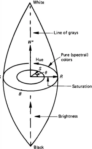
Figure 3.10 Perceptual representation of the color space. The brightness W*

varies along the vertical axis, hue 0 varies along the circumference, and saturation S

1 00

80

c 0

·;:;

e- ₆₀

0

1l _cu ,( _{"' 40}

E ... ₀

11'-20

0

400

S3 (X)

J S1 (A.)C(X)dA. _{°'1 (C)}

450 500 550 600 650

Wavelength (nm)

(a) Typical sensitivity curves for _{S1 , S2, S3}

(not to scale). (b) Three receptor model for color representation

Figure 3.11 (a) Typical absorption spectra of the three types of cones in the human retina; (b) three-receptor model for color representation.

hues are manifested by the differences in wavelengths. Saturation is that aspect of perception that varies most strongly as more and more white light is added to a monochromatic light. These definitions are somewhat imprecise because hue, satur­ ation, and brightness all change when either the wavelength, the intensity, the hue, or the amount of white light in a color is changed. Figure 3 . 10 shows a perceptual representation of the color space. Brightness (W* ) varies along the vertical axis, hue (0) varies along the circumference, and saturation (S) varies along the radial distance. t For a fixed brightness W*, the symbols R, G, and B show the relative

locations of the red, green, and blue spectral colors.

Color representation is based on the classical theory of Thomas Young (1802) [8] , who stated that any color can be reproduced by mixing an appropriate set of three primary colors. Subsequent findings, starting from those of Maxwell [9] to more recent ones reported in [10, 11] , have established that there are three different types of cones in the (normal) human retina with absorption spectra S1(A), S2(A), and S3(A), where Amin :5 A :5 Amax , Amin = 380 nm, Amax = 780 nm. These responses

peak in the yellow-green, green, and blue regions, respectively, of the visible electromagnetic spectrum (Fig. 3. lla). Note that there is significant overlap between S1 and S2 .

Based on the three-color theory, the spectral energy distribution of a "colored" light, C(A), will produce a color sensation that can be described by

spectral responses (Fig. 3. llb) as

J�max

o:; (C) = S; (A)C(A) dA, >i.min

i = 1 , 2, 3 (3. 18)

' The superscript • used for brightness should not be confused with the complex conjugate. The notation used here is to remain consistent with the commonly used symbols for color coordinates.

Equation

(3.18)

may be interpreted as an equation of color representation. If

C1(A.)

and

Ci(A.)

are two spectral distributions that produce responses o:;

( C1)

and o:;

( C2)

such that

i

=

1, 2, 3

(3.19)

then the colors

C1

and

C2

are perceived to be identical. Hence two colors that look identical could have different spectral distributions.

3.8 COLOR MATCHING AND REPRODUCTION

One of the basic problems in the study of color is the reproduction of color using a set of light sources. Generally, the number of sources is restricted to three which, due to the three-receptor model, is the minimum number required to match arbitrary colors. Consider three primary sources of light with spectral energy distri­ butions

Pk(A.),

k

=

1, 2, 3.

Let

(3.20)

where the limits of integration are assumed to be

Amin

and

Amax

and the sources are linearly independent, i.e . , a linear combination of any two sources cannot produce the third source. To match a color

C(A),

suppose the three primaries are mixed in

3

proportions of

13k>

k

=

1, 2, 3

₍Fig.

3.12).

Then L

13k Pk(A)

should be perceived as

C(�) .

I\. ' i.e. '

k=I

o:;(C) = J[kt113kPk(A)]S;(A)dA= J113kf S;(A)Pk(A)dA

i

= 1,2,3 (3.21)

Defining the ith cone response generated by one unit of the kth primary as

i,k

=

l

,2,

3

(3.22)

we get

±

13ka;,k=o:;(C) = J S;(A)C(A)dA,

k=l

i =

1,2,3

(3.23)

These are the color matching equations. Given an arbitrary color spectral distribu­ tion

C(A),

the primary sources

Pk(A),

and the spectral sensitivity curves S;

(A),

the quantities

13k,

k

= 1, 2, 3,

can be found by solving these equations. In practice, the primary sources are calibrated against a reference white light source with known

energy distribution W(A.). Let _wk denote the amount of kth primary required to match the reference white. Then the quantities

T. k (C) = 13k

wk ' k

=

1 , 2, 3 (3.24)

are called the tristimulus values of the color C. Clearly, the tristimulus values of the reference white are unity. The tristimulus values of a color give the relative amounts of primaries required to match that color. The tristimulus values, Jk(A.), of unit energy spectral color at wavelength A. give what are called the spectral matching

curves. These are obtained by setting C(A.)

=

B(A. - A.') in (3.23), which together with (3.24) yield three simultaneous equations

3

L wk a;, k Tk(A.')

=

S; (A.'), i

=

1 , 2, 3 (3.25)

k=I

for each A.' . Given the spectral tristimulus values 7k(A.), the tristimulus values of an arbitrary color C(A.) can be calculated as (Problem 3.8)

1k(C)

=

I

C(A.)Tk(A.) dA., k = 1 , 2, 3 (3.26)

Example 3.1

The primary sources recommended by the CIE• as standard sources are three monochromatic sources

P1(>..) = _{8(>.. - >..1),} P2(>..) = 8(>.. - >..2), PJ(>..) = 8(>.. -A3),

>..1 = 700 nm, red

>..2 = 546.l nm, green

A3 = 435.8 nm, blue

Using (3.22), we obtain a;, k = S; (>..k), i, k = 1, 2, 3. The standard CIE white source has a

flat spectrum. Therefore, a;(W) = fS; (>..)d>... Using these two relations in (3.23) for reference white, we can write

±

wk S; (>..k) =

J

S; (>..) d>..,

k = l i = 1 , 2, 3 (3.27)

which can be solved for wk provided {S; (>..k), 1 :s i, k :s 3} is a nonsingular matrix. Using the spectral sensitivity curves and wk , one can solve (3.25) for the spectral tristimulus values Tk(>..) and obtain their plot as in Fig. 3.13. Note that some of the tristimulus values are negative. This means that the source with negative tristimulus value, when mixed with the given color, will match an appropriate mixture of the other two sources. It is safe to say that any one set of three primary sources cannot match all the visible colors; although for any given color, a suitable set of three primary sources can be found. Hence, the primary sources for color reproduction should be chosen to maximize the number of colors that can be matched.

Laws of Color Matching

The preceding theory of colorimetry leads to a useful set of color matching rules [13] , which are stated next.

' Commission Internationale de L'Eclairage, the international committee on color standards.

0.4

T1 Pd

0.3

"'

QJ :J _0.2

.... >

"'

2

:J

E _0.1

:; .=

0

-0. 1

Wavelength, X(nm)

Figure 3.13 Spectral matching tristimulus curves for the CIE spectral primary system. The negative tristimulus values indicate that the colors at those wavelengths cannot be reproduced by the CIE primaries.

1.

Any color can be matched by mixing at most three colored lights. This means we can always find three primary sources such that the matrix {a;, k} is non­ singular and (3.23) has a unique solution.

2.

The luminance of a color mixture is equal to the sum of the luminances of its

components. The luminance Y of a color light C(>..) can be obtained via (3.2) as (here the dependence on x, y is suppressed)

y

=

Y(C) =

I

C(>..)V(>..) d>.. (3.28) From this formula, the luminance of the kth primary source with tristimulus setting �k = wk 1k (see Fig. 3.12) will be Tk wk f Pk(>..)V(>..) d>... Hence the lumi­ nance of a color with tristimulus values 1k , k = 1 , 2, 3 can also be written as

3 3

Y = L

Ikf

wk Pk(>..)V(>..) d>..� L Tk lk (3.29)

k=l k= l

where h is called the luminosity coefficient of the kth primary. The reader should be cautioned that in general

3

C(>..) -=f. L wk TkPk(>..)

k= l

even though a color match has been achieved.

(3.30)

3. The human eye cannot resolve the components of a color mixture. This means that a monochromatic light source and its color are not unique with respect to each other, i.e. , the eye cannot resolve the wavelengths from a color.

5. Color addition:

If a color C1 matches color C2 and a color c; matches color CZ ,

then the mixture of C1 _{and c; matches the mixture of} C2 _and C]. . Using the notation

[Ci] = [ C2] � color C1 matches color C2

a1( C1] + a2( C2] � a mixture containing an amount a1 of C1 and an amount a1 of C2

we can write the preceding law as follows. If

(Ci] = (Ci] and (C2] = (C2]

then

6.

Color subtraction:

If a mixture of C1 and C2 matches a mixture of Cl and C]. and

if C2 _matches C]. _then C1 _matches Ci , i.e. , if

(Ci] + (C2] = (Cl] + (CZ]

and (C2] = (CZ]

then (Ci] = (Cl]

7.

Transitive law:

If C1 matches C2 and if C2 matches C3 , then C1 matches C3 ,

i.e . , if

then

8.

Color matches:

Three types of color matches are defined:

a. a(C] = a1(Ci] + a2[C2] + a3(C3]; i.e . , a units of C are matched by a mixture of a1 units of C1 , a2 units of C2 , and a3 units of C3 . This is a direct match. Indirect matches are defined by the following.

b. a( C] + a1( Ci] = a1[ C2] + a3( C3]

c. a(C] + a1(Ci] + a1(C2] = a3(C3]

These are also called Grassman's laws. They hold except when the luminance levels are very high or very low. These are also useful in color reproduction colorimetry, the science of measuring color quantitatively.

Chromaticity Diagram

The chromaticities of a color are defined as

k = 1, 2, 3 (3.31)

Clearly t1 + t2 + t3 = l. Hence, only two of the three chromaticity coordinates are independent. Therefore, the chromaticity coordinates project the three­ dimensional color solid on a plane. The chromaticities t1 , t2 jointly represent the

g

-0.5 Line of purples

Figure 3.14 Chromaticity diagram for the CIE spectral primary system. Shaded area is the color gamut of this system.

chrominance components (i.e. , hue and saturation) of the color. The entire color space can be represented by the coordinates (t1 , t2 , Y), in which any Y = constant is a chrominance plane. The chromaticity diagram represents the color subspace in the chrominance plane. Figure 3 . 14 shows the chromaticity diagram for the CIE spectral primary system. The chromaticity diagram has the following properties:

1.

The locus of all the points representing spectral colors contains the region of all the visible colors.

2. The straight line joining the chromaticity coordinates of blue (360 nm) and red (780 nm) contains the purple colors and is called the line of purples.

3. The region bounded by the straight lines joining the coordinates (0, 0), (0, 1) and (1, 0) (the shaded region of Fig. 3. 14) contains all the colors reproducible by the primary sources. This region is called the color gamut of the primary sources.

4. The reference white of the CIE primary system has chromaticity coordinates

(t �).

Colors lying close to this point are the less saturated colors. Colors located far from this point are the more saturated colors. Thus the spectral colors and the colors on the line of purples are maximally saturated.

3.9 COLOR COORDINATE SYSTEMS

TABLE 3.4 Color Coordinate Systems

Color coordinate system

1 . C. /. E. spectral primary system: R, G, B

2. C.I. E. X, Y, Z system Y = luminance

3. C.l. E. uniform chromaticity scale (UCS) system: u, v, Y

u, v = chromaticities

Y = luminance

U, V, W = tristimulus

values corresponding to

u, v, w

4. u·' v·. w· system (modified UCS system)

Y = luminance (0.01 , I)

5. s . 0, w· system: S = saturation

e = hue

w• = brightness

6. NTSC receiver primary system R

N

, GN, BN

7. NTSC transmission system: Y = luminance

I, Q = chrominances

8. L * , a', b* system:

L • = brightness

a • = red-green content

b • = yellow-blue content

Description

Monochromatic primary sources P, , red = 700 nm,

P,, green = 546. l nm, P,, blue = 435.8 nm. Reference

white has flat spectrum and R = G = B = l . See Figs.

3 . 1 3 and 3 . 14 for spectral matching curves and

chromaticity diagram .

[�]

=

[�:i�� �:�!� �:���] [�]

Z 0.000 0.010 0.990 B

4X 4x

u = -- --- - --- =

----x + 15Y + 3Z -2x + 1 2y + 3

6Y 6y

v = _{X-+--15_Y_+-3Z = - 2x-+�12_y_+�3}

U =2}(_ V = Y W =- X + 3 Y + Z

3 ' ' 2

U* = 13W *(u -Uo)

v· = 1 3 W * ( v -Vo)

w• = 25( 100Y)"' - 17, J s lDOY s 100 u0, v0 = chromaticities of reference white

w· = contrast or brightness

S = [( U *)' + ( V *)'J"' = 13W *[(u - Uo)' + (v -

Vo)']"'

0=tan-' (�:)

= tan - ' [(v - vo)/(u - uo)], O s 0 S 2ir

Linear transformation of X, Y, Z. Is based on

television phosphor primaries. Reference white is illuminant C for which R:v = GN = BN = l .

[RN] [

i .910 -0.533 -0.288

][

x

]

GN = -0.985 2.000 -0.028 y

BN 0.058 - 0 . 1 18 0.896 z

Y = 0.299RN + 0.587G:v +-0. 1 14B:v I = 0.596R:v - 0.274GN - 0.3228..,,

Q = 0.21 I R..., -0.523GN + 0.312B:v

L • = 25

(

lO

�

,

y

)

_{"' - 16, 1 s lDOY s 100}

• _{_}

[(

X

)

''·'

(

Y

)

"-'

]

a - 500 -

-Xo Y,,

• _-

[

(

y

)

''-'

(

z

)

'''

]

b - 200 - -

-Y,, Zo

X11, Y,,, Z0 = tristimulus values of the reference white

As mentioned before, the CIE spectral primary sources do not yield a full gamut of reproducible colors. In fact, no practical set of three primaries has been found that can reproduce all colors. This has led to the development of the CIE X, Y, Z system with hypothetical primary sources such that all the spectral tri­

stimulus values are positive. Although the primary sources are physically unreal­ izable, this is a convenient coordinate system for colormetric calculations. In this system Y represents the luminance of the color. The X, Y, Z coordinates are related to the CIE R, G, B system via the linear transformation shown in Table 3.4. Figure 3.15 shows the chromaticity diagram for this system. The reference white for this system has a flat spectrum as in the R, G, B system. The tristimulus values for the reference white are X

=

Y

=

Z

=

1 . ·

Figure 3.15 also contains several ellipses of different sizes and orientations. These ellipses, also called MacAdam ellipses [10, 1 1 ] , are such that colors that lie inside are indistinguishable. Any color lying just outside the ellipse is just

noticeably different (JND) from the color at the center of the ellipse. The size, orientation, and eccentricity (ratio of major to minor area) of these ellipses vary throughout the color space. The uniform chromaticity scale (UCS) system u, v, Y transforms these elliptical contours with large eccentricity (up to 20 : 1) to near circles (eccentricity = 2 : 1) of almost equal size in the u, v plane. It is related to the X, Y, Z system via the transformation shown in Table 3.4. Note that x, y and u, v are

the chromaticity coordinates and Y is the luminance. Figure 3 . 16 shows the chromaticity diagram of the UCS coordinate system. The tristimulus coordinates corresponding to u, v, and

w

� 1

-

u

-

v are labeled as U, V, and W respectively. The U*, V*, W* system is a modified UCS system whose origin (u0 , v0

)

is

shifted to the reference white in the u, v chromaticity plane. The coordinate W* is a cube root transformation of the luminance and represents the contrast (or

0.8

0.6

0.4

0.2 v

520

Figure 3.15 Chromaticity diagram for the CIE XYZ color coordinate system.

1..-.L-..L--"llli:;;.&...J...J...L---L---1---1L--L-.L-.L-...L...-x The (MacAdam) ellipses are the just

brightness) of a uniform color patch. This coordinate system is useful for measuring color differences quantitatively. In this system, for unsaturated colors, i.e. , for colors lying near the grays in the color solid, the difference between two colors is, to a good approximation, proportional to the length of the straight line joining them. The S, 6, W* system is simply the polar representation of the U*, V*, W* system, where S and 6 represent, respectively, the saturation and hue attributes of color (Fig. 3.10). Large values of S imply highly saturated colors.

The National Television Systems Committee (NTSC) receiver primary system

(RN , GN , BN)

was developed as a standard for television receivers. The NTSC has adopted three phosphor primaries that glow in the red, green, and blue regions of the visible spectrum. The reference white was chosen as the illuminant C, for which the tristimulus values are

RN = GN = BN =

1 . Table 3.5 gives the NTSC coordinates of some of the major colors. The color solid for this coordinate system is a cube (Fig. 3. 17). The chromaticity diagram for this system is shown in Fig. 3 .18. Note that the reference white for NTSC is different from that for the CIE system.

The NTSC transmission system (Y, I, Q ) was developed to facilitate trans­ mission of color images using the existing monochrome television channels without increasing the bandwidth requirement. The Y coordinate is the luminance (mono­ chrome channel) of the color. The other two tristimulus signals, I and Q, jointly represent hue and saturation of the color and whose bandwidths are much smaller than that of the luminance signal. The /, Q components are transmitted on a subcarrier channel using quadrature modulation in such a way that the spatial

TABLE 3.5 Tristimulus and Chromaticity Val ues of Major Colors in the NTSC

Receiver Primary System

Red Yellow Green Cyan Blue Magenta White Black

RN 1.0 1.0 0.0 0.0 0.0 1.0 1.0 0.0

GN 0.0 1.0 1.0 1.0 0.0 0.0 1.0 0.0

BN 0.0 0.0 0.0 1.0 1.0 1.0 1.0 0.0

YN 1.0 0.5 0.0 0.0 0.0 0.5 0.333 0.333

gN 0.0 0.5 1.0 0.5 0.0 0.0 0.333 0.333

bN 0.0 0.0 0.0 0.5 1.0 0.5 0.333 0.333

BN

Green _Yellow

81 ue Magenta

500

�----ii---800

360

Line of purples

Figure 3.17 Tristimulus color solid for the NTSC receiver primary system.

Figure 3.18 Chromaticity diagram for the NTSC receiver primary system.

spectra of I, Q do not overlap with that of Y and the overall bandwidth required for transmission remains unchanged (see Chapter 4). The Y, I, Q system is related to the RN , GN , BN system via a linear transformation. This and some other trans­ formations relating the different coordinate systems are given in Table 3.6.

The L *, a*, b* system gives a quantitative expression for the Munsell system of color classification [12]. Like the U*, V*, W* system, this also gives a useful color difference formula.

Example 3.2

We will find the representation of the NTSC receiver primary yellow in the various coordinate systems. From Table 3.5, we have RN = 1.0, GN = 1.0, BN = 0.0.

Using Table 3.6, we obtain the CIE spectral primary system coordinates as R = 1.167 - 0.146 - 0.0 = 1.021, G = 0.114 + 0.753 + 0.0 = 0.867, B = -0.001 +

0.59 + 0.0 = 0.058.

The corresponding chromaticity values are

r ₌ 1.021 ₌ 0.525

1.021 + 0.867 + 0.058 '

g

= 0.867 = 0.445

1.946 ' b = 0·058 = 0.030

1.946 Similarly, for the other coordinate systems we obtain:

x = 0.781, y = 0.886, z = 0.066; u = 0.521, v = 0.886, w = 0.972,

y = 0.886, I = 0.322, Q = -0.312

x = 0.451, y = 0.511,

u = 0.219, v = 0.373,

z = 0.038

w =

0.408

TABLE 3.6 Transformations from NTSC Receiver Primary to Different Coordinate

Systems. I nput Vector is _{[RN GN BNY·}

Output

vector Transformation matrix Comments

m

(

1.161 -0.146 -0.151

)

0.114 0.753 0.159 CIE spectral primary system

-0.001 0.059 1.128

m

(

0.607 0.174 0.201

)

0.299 0.587 0.114 CIE X, Y, Z system

0.000 0.066 1.117

[!]

(

0.405 0.116 0.133

)

0.299 0.587 0.114 CIE UCS tristimulus system

0.145 0.827 0.627

m

(

0.299 0.587 0.114

)

0.596 -0.274 -0.322 NTSC transmission system

0.211 -0.523 0.312

not unity because the reference white for NTSC sources is different from that of

the CIE. Using the definitions of

u

and

v

from Table 3.4, we obtain

u0 =

0.201,

v0

=

0.307 for the reference white.

Using the preceding results in the formulas for the remaining coordinate

systems, we obtain

W*

=

25(88.6)1'3 - 17

=

94.45,

U* =

22.10,

V*

=

81.04

S =

84.00,

0 =

tan-1(3.67)

=

1.30 rad,

W* =

94.45

L * =

25(88.6)113 - 16

=

95 .45,

a*

=

500[

(�: ���r3

-

(0·�86)1'3]

=

-16. 98

b* =

200[ (0.886)1'3 -

(�:���)

113]

=

115.67

3.10 COLOR DIFFERENCE MEASURES

Quantitative measures of color difference between any two arbitrary colors pose a

problem of considerable interest in coding, enhancement, and analysis of color

images. Experimental evidence suggests that the tristimulus color solid may be

considered as a Riemannian space with a color distance metric [14, 15]

3 3

(ds)2 = _{2: 2:} C;,j dX; dXj

i = l j = 1

(3.32)

The distance

ds

represents the infinitesimal difference between two colors with

coordinates

X;

and

X; + dXi

in the chosen color coordinate system. The coefficients

C;, i

measure the average human perception sensitivity due to small differences in the

ith and in the jth coordinates.

Small differences in color are described on observations of

just noticeable

differences (JNDs)

in colors.

A

unit

JND

defined by

3 3

1

=

2: 2: C;,jdX;dXj

i = l j = I (3.33)

is the describing equation for an ellipsoid. If the coefficients

c;,i

were constant

throughout the color space, then the

JND

ellipsoids would be of uniform size in

the color space. In that event, the color space could be reduced to a

Euclidean

tristimulus space,

where the color difference between any two colors would become

proportional to the length of the straight line joining them. Unfortunately, the

C;,i

exhibit large variations with tristimulus values, so that the sizes as well as

the orientations of the

JND

ellipsoids vary considerably. Consequently, the distance

between two arbitrary colors

C1

and

C2

is given by the minimal distance chain of

ellipsoids lying along a curve

�*

joining

C1

and

C2

such that the distance integral

Ll

1C2(X;)

d(Ci

,

C2) =

�J,

C1(X;)

ds (3.34)

is minimum when evaluated along this curve, i.e., for

�

=

�*.

This curve is called

the

geodesic

between

C1

and

C2 .

If

c;, i

are constant in the tristimulus space, then the

geodesic is a straight line. Geodesics in color space can be determined by employing

a suitable optimization technique such as dynamic programming or the calculus of

v

0.4 Green

0.3

0.2

0.1

0 0.1

Blue

0.2 0.3 0.4 0.5

TABLE 3.7 CIE Color-Difference Formu las

Formula

(.:is)2 = (6.U *)2 + (6.V *)2 + (6.W*)2 (.:is)2 = (6.L *)2 + (6.u *)2 + _{(6.v *)2}

L * = 25

(

1

�

Y

r

3 - 16

u * = 13L * (u ' - u0) v * = 13L * ( v ' - v0) u ' = u

I 1 5 9Y

v = . v =

X + 15 Y + 3Z

(.:is)2 = (6.L *)2 + (6.a *)2 + (M _*)2

Equation Number

(3.35) (3.36)

(3.37)

Comments

1964 CIE formula

1976 CIE formula, modification of

the u, v, Y space to u *, v *, L *

space. uo, Vo, Yo refer to reference white.

L * , a * , b * color coordinate

system.

vanatlons [15]. Figure 3.19 shows the projections of several geodesic curves

between the major NTSC colors on the UCS

_{u, v}

chromaticity plane. The geodesics

between the primary colors are nearly straight lines (in the chromaticity plane), but

the geodesics between most other colors are generally curved.

Due to the large complexity of the foregoing procedure of determining color

distance, simpler measures that can easily be used are desired. Several simple

formulas that approximate the Riemannian color space by a Euclidean color space

have been proposed by the CIE (Table 3.7). The first of these formulas [eq. (3.35)]

was adopted by the CIE in 1964. The formula of (3.36), called the CIE 1976

L *, u*, v*

formula, is an improvement over the 1964 CIE

U*, V*, W*

formula in

regard to uniform spacing of colors that exhibit differences in sizes typical of those

in the Munsell

book of color

[12].

The third formula, (3.37), is called the CIE 1976

L *, a*, b*

color-difference

formula. It is intended to yield perceptually uniform spacing of colors that exhibit

color differences greater than JND threshold but smaller than those in the Munsell

book of color.

3.1 1 COLOR VISION MODEL

With color represented by a three-element vector, a color vision model containing

three channels [16], each being similar to the simplified model of Fig. 3.9, is shown

in Fig. 3.20. The color image is represented by the

RN , GN , BN

coordinates at

each pixel. The matrix

A

transforms the input into the three cone responses

o'.k(x, y, C), _k

= 1, 2, 3, where

(x, y)

are the spatial pixel coordinates and

C

refers to

its color. In Fig. 3.20, we have re

p

resented the

normalized cone responses

T' d ak(x, y, C)

k = ak(x, y, _{W) '}

k = l,2,3

(3.38)

RN (x, vi r,·(x, vi _7', c, (x, vi

H1 (t1 , bl 81 (x, vi

GN (x, vl Ti(x, vi _7'2 C2 (x, vi

A B H2 !t, , E21 B2 (x, vi

BN (x, vl Tj(x, vi _7'3 C3 (X, vi

H3 (E, ' E21 B3 (x, vi

Figure 3.20 A color vision model.

In analogy with the definition of tristimulus values,

Tk

are called the

retinal

cone

tristimulus coordinates

(

see Problem 3.14

)

. The cone responses undergo non­

linear point transformations to give three fields

Tk(x, y), k =

1, 2, 3. The 3

x

3 matrix

B

transforms the

{f(x, y)}

into

{Ck(x, y)}

such that

C1(x, y)

is the monochrome

(

achromatic

)

contrast field

c(x, y),

as in Fig. 3.9, and

C2(x, y)

and

C3(x, y)

represent

the corresponding chromatic fields. The spatial filters

Hk(�1 , �2), k

=

1, 2, 3, repre­

sent the frequency response of the visual system to luminance and chrominance

contrast signals. Thus

H1(�1 , �2)

is the same as

H (�1 , �2)

in Fig. 3.9 and is a band­

pass filter that represents the lateral inhibition phenomenon. The visual frequency

response to chrominance signals are not well established but are believed to have

their passbands in the lower frequency region, as shown in Fig. 3.21. The 3 x 3

matrices

A

and

B

are given as follows:

(

0.299 0.587 0.114

)

A =

-0.127 0.724 0.175 ,

0.000 0.066 1.117

(

21.5 0.0 0.00

)

B =

-41.0 41.0 0.00

- 6.27 0.0 6.27

(

3.39

)

From the model of Fig. 3.20, a criterion for color image fidelity can be

defined. For example, for two color images

{RN , GN , BN}

and

{R,,V, G,,V, BN},

their

sub

j

ective mean square error could be defined by

e1s = l_

± J

f

(Bk(x, y) - Bk(x, y))2 dx dy

A k=I

Jell

(

3.40

)

where

<!ft

is the region over which the image is defined

(

or available

)

,

A

is its area,

and

{Bk(x, y)}

and

{Bk(x, y)}

are the outputs of the model for the two color images.

1 . 0

0. 1 .__ _ __. _ __.. __ __.. _ _._...__,___,'---i� p 0.1 0.3 1 .0 3.0 1 0.0

Cycles/degree

30.0

Figure 3.21 Frequency responses of the three color channels Ci. C2, C3 of the color vision model. Each filte_X is assumed to be isotropic so that Hpk (p) = Hk ( �i. �),

3.12 TEMPORAL PROPERTIES OF VISION

Temporal aspects of visual perception

[1 , 18]

become important in the processing of

motion images and in the design of image displays for stationary images. The main

properties that will be relevant to our discussion are summarized here.

Bloch's Law

Light flashes of different durations but equal energy are indistinguishable below a

critical duration. This critical duration is about

30

ms when the eye is adapted at

moderate illumination level. The more the eye is adapted to the dark, the longer is

the critical duration.

Critical Fusion Frequency (CFF)

When a slowly flashing light is observed, the individual flashes are distinguishable.

At flashing rates above the

critical fusion frequency

(CFF), the flashes are indistin­

guishable from a steady light of the same average intensity. This frequency gener­

ally does not exceed

50

to

60

Hz. Figure

3.22

shows a typical temporal MTF.

This property is the basis of television raster scanning cameras and displays.

Interlaced image fields are sampled and displayed at rates of

50

or

60

Hz. (The rate

is chosen to coincide with the power-line frequency to avoid any interference.) For

digital display of still images, modern display monitors are refreshed at a rate of

60

frames/s to avoid any flicker perception.

Spatial versus Temporal Effects

The eye is more sensitive to flickering of high spatial frequencies than low spatial

frequencies. Figure

3.22

compares the temporal MTFs for flickering fields with

different spatial frequencies. This fact has been found useful in coding of motion

� ·;;

1 .0

0.5

·;::; 0.2

·;;;

& � 0.1

·;::;

IU

� 0.05

0.02

High spatial

-frequencies field Low spatial

-- frequencies field

0.01 L--....L.-L--....l..--..1...----L--.I.-�

2 5 1 0 20 50

Flicker frequency ( Hz)

Sec. 3.1 2 Temporal Properties of Vision

Figure 3.22 Temporal MTFs for flicker­ ing fields.

images by subsampling the moving areas everywhere except at the edges. For the same reason, image display monitors offering high spatial resolution display images at a noninterlaced 60-Hz refresh rate.

P R O B L E M S

3.1 Generate two 256 x 256 8-bit images as in Fig. 3.3a, where the small squares have gray level values of 127 and the backgrounds have the values 63 and 223. Verify the result of Fig. 3.3a. Next change the gray level of one of the small squares until the result of Fig. 3.3b is verified.

3.2 Show that eqs. (3.5) and (3.6) are solutions of a modified Weber law: df If"" is

pro­

portional todc,

i.e., equal changes in contrast are induced by equal amounts of df/f �.

Find -y.

3.3 Generate a digital bar chart as shown in Fig. 3.5a, where each bar is 64 pixels wide. Each image line is a staircase function, as shown in Fig. 3.5b. Plot the brightness function (approximately) as you perceive it.

3.4 Generate a 512 x 512 image, each row of which is a smooth ramp

r(n)

as shown in

Fig. P3.4. Display on a video monitor and locate the dark (D ) and the bright (B) Mach bands.

r(n)

240 225

1 35

1 20 �----�

1 00 200 280 300 51 2

Figure P3.4

3.5 The Mach band phenomenon predicts the one-dimensional step response of the visual

system, as shown by

s(n)

in Fig. P3.5. The corresponding one-dimensional impulse response (or the vertical line response) is given by

h(n) =s(n)-s(n

- 1). Show that

h(n)

has negative lobes (which manifest the lateral inhibition phenomenon) as shown in Fig. 3.6c.

3.6 As a rule of thumb, the peak-to-peak value of images can be estimated as

nu,

where

n

varies between 4 to 6. Letting

n

= 5 and using (3.13), show that

0.5

2.7

,f-. ... 2.5

I I ... ---.... -• -- Step response s(n) I I 1 _I

I I I I

I I I _I

2.0 .,__...._--.--+---Step input

I

1 .0

;

, 1 I I I I _I

' I I

'f

0.3

:

I

I

I

I

I

I

-3 -2 -1 0 2

Figure P3.5

3.7 Can two monochromatic sources with different wavelengths be perceived to have the same color? Explain.

3.8 Using eqs. (3.23) through (3.25), show that (3.26) is valid.

3.9 In this problem we show that any two tristimulus coordinate systems based on different sets of primary sources are linearly related. Let {Pk(A.)} _and {P,;(A.)}, _k = 1, 2, 3, be two

sets of primary sources with corresponding tristimulus coordinates {Tk} _and {T,;} _and

reference white sources W(A.) _and W' (A.). _{If a color} C (A.) _{is matched by these sets of}

sources, then show that

3 3

L a;, kwk Tk(C) = L a/ k w,; T,;(C)

k = I k = I

where the definitions of a's and w's follow from the text. Express this in matrix form and write the solution for {T,;}.

3.10 Show that given the chromaticities 11 , 12 and the luminance Y, the tristimulus values of a coordinate system can be obtained by

tk y

Tk =

-3--L

t; t;

j rz ]

k = 1 , 2, 3

where !, are the luminosity coefficients of the primary sources.

3.11* For all the major NTSC colors listed in Table 3.5, calculate their tristimulus values in the RGB, XYZ, UVW, YIQ, U* V*W, L*a*b*, S 0W*, and Ti Ti Tj coordinate

systems. Calculate their chromaticity coordinates in the first three of these systems. 3.12 Among the major NTSC colors, except for white and black (see Table 3.5), which one

(a) has the maximum luminance, (b) is most saturated, and (c) is least saturated? 3.13* Calculate the color differences between all pairs of the major NTSC colors listed in

Table 3.5 according to the 1964 CIE formula given in Table 3.7. Which pair of colors is (a) maximally different, (b) minimally different? Repeat the calculations using the

L *a*b* system formula given by (3.37).

3.14 [Retinal cone system; Ti , Ti , Tj] Let Pk(;>..), k = 1, 2, 3 denote the primary sources

that generate the retinal cone tristimulus values. Using (3.38), (3.24) and (3.23), show that this requires (for every x, y, C)

3

L ak(x, y, C)a,, k = a,(x, y, C) :::} a,, k = &(i - k)

k= I

To determine Pk(;>..), write

3

Pk(A) = _{i= I}

L

S,(;>..)bi, k ' k = l, 2 , 3 and show that (P3.14) implies B

�

{b,, k} =

:I-1,

where

:I �

{er,) and

CTi, j =

J

S,(;>..)Sl;>..) d;>..

Is the set {Pk(A)} physically realizable? (Hint: Are b,, k nonnegative?)

B I B L I O G R A P H Y

Sections 3.1-3.3

For further discussion on fundamental topics in visual perception:

1. T. N. Cornsweet. Visual Perception. New York: Academic Press, 1971.

(P3.14)

2. E. C. Carterette and M. P. Friedman, eds. Handbook of Perception, vol. 5. New York: Academic Press, 1975.

3. S. Hecht. "The Visual Discrimination of Intensity and the Weber-Fechner Law."

J. Gen. Physiol. 7, (1924): 241.

Section 3.4

For measurement and applications of the visibility function:

4. A. N. Netravali and B. Prasada. "Adaptive Quantization of Picture Signals Using Spatial Masking." Proc. IEEE 65, (April 1977): 536-548.

Sections 3.5-3.6

For a detailed development of the monochrome vision model and related image

fidelity criteria:

5. C. F. Hall and E. L. Hall. "A Nonlinear Model for the Spatial Characteristics of the Human Visual System." IEEE Trans. Syst. Man. Cybern., SMC-7, 3 (March 1977): 161-170.

6. J. L. Mannos and D. J. Sakrison. "The Effects of a Visual Fidelity Criterion on the Encoding of Images." IEEE Trans. Info. Theory IT-20, no. 4 (July 1974): 525-536. 7. D. J. Sakrison. "On the Role of Observer and a Distortion Measure in Image Trans­

Sections 3.7-3 . 1 0

For introductory material on color perception, color representation and general

reading on color:

8. T. Young. "On the Theory of Light and Colors." Philosophical Transactions of the Royal Society of London, 92, (1802): 20-71.

9. J. C. Maxwell. "On the Theory of Three Primary Colours." Lectures delivered in 1861. W. D. Nevin (ed.), Sci. Papers 1, Cambridge Univ. Press, London (1890): 445-450.

10. D. L. MacAdam. Sources of Color Science. Cambridge, Mass.: MIT Press, 1970.

11. G. W. Wyzecki and W. S. Stiles. Color Science. New York: John Wiley, 1967. 12. Munsell Book of Color. Munsell Color Co., 2441 North Calvert St., Baltimore, Md. 13. H. G. Grassman. "Theory of Compound Colours." Philosophic Magazine 4, no. 7

(1954): 254-264.

For color distances, geodesics, and color brightness:

14. C.l.E. "Colorimetry Proposal for Study of Color Spaces" (technical note). J. Opt. Soc.

Am. 64, (June 1974): 896-897.

15. A. K. Jain. "Color Distance and Geodesics in Color 3 Space." J. Opt. Soc. Am. 62 (November 1972): 1287-1290. Also see J. Opt. Soc. Am. 63, (August 1973): 934-939.

Section 3.1 1

For the color vision model, their applications and related biography:

16. W. Frei and B. Baxter. "Rate Distortion Coding Simulation for Color Images." IEEE Trans. Communications COM-25, (November 1977): 1385-1392.

17. J. 0. Limb, C. B. Rubinstein, and J. E. Thompson. "Digital Coding of Color Video Signals." IEEE Trans. Communications COM-25 (November 1977): 1349-1384.

Section 3.12

For further details on temporal visual perceptions, see [1] and:

18. D. H. Kelly. "Visual Responses to Time Dependent Stimuli. I. Amplitude Sensitivity Measurements." J. Opt. Soc. Am. 51, (1961): 422-429. Also see pp. 917-918 of this

issue, and Vol. 59 (1969): 1361-1369.