Assessing impacts of small perturbations using a model-based
approach
Michael B. Dale
a, Patricia E.R. Dale
a,*
, Cen Li
b, Gautam Biswas
ca
Griffith University, Australian School of Environmental Studies, Nathan 4111, Queensland, Australia
b
Department of Electrical Engineering and Computer Science, Middle Tennessee State University, Murfreesboro, TN, USA
c
Department of Computer Science, Vanderbilt University, TN, USA
Received 28 November 2001; received in revised form 26 April 2002; accepted 8 May 2002
Abstract
When examining the effects of a disturbance on a complex system likevegetation it is difficult to distinguish between those changes that affect the processes underlying the functioning of the system and other changes which simply shift the state of the system but have no effect on the processes. The former is obviously a more significant effect than the latter. In this paper we examine a model-based clustering procedure which can make such a distinction. Given observations on several sites on several occasions, we model the dynamics of the processes using a continuous hidden Markov model. In this model the actual Markov process is hidden, but at any observation time we can observe surrogatevariables whosevalues will be conditional on the underlying state of the process. We further ask if there is evidence for more than one such process, i.e. whether our data are heterogeneous. By estimating the number of clusters using a Bayesian information criterion we can choose between these alternatives. An analogous assessment is made of the number of states in the underlying hidden Markovmodels, as well as the transition matrices between states and emission probabilities relating the underlying hidden state to the observed attributes. The methodology was applied to the question of determining if a runnelling treatment of a salt marsh for mosquito management had changed the underlying processes related to thevegetation.# 2002 Elsevier Science B.V. All rights reserved.
Keywords: Hidden Markovmodels; Model-based clustering; Salt marshes; Runnelling
1. Introduction
Assessing the impact of disturbance onv egeta-tion is a critical activity, for vegetation reflects
general environmental conditions and should in-dicate the cumulative effects of change. In some cases the impact is so large that there can be little need for sophisticated assessment: clearing of a forest can hardly be regarded as other than an obvious and major impact. Yet a destructive fire in a Eucalyptus regnans F. Muell. forest can cause equally massive changes but is a necessary part of the process of regeneration and as such represents only a change of state and not a change of process. Abbreviations: MML, minimum message length; HMM,
hidden Markovmodel; BIC, Bayesian information criterion. * Corresponding author. Tel.:/61-7-3875-7136; fax: /61-7-3875-7616
E-mail address: [email protected](P.E.R. Dale).
When dealing with less intrusive activities, with more delicate manipulations, the assessment of impact itself becomes a delicate procedure. There are experimental designs for assessing impact, such as ‘Before After Control Intervention’ (Faith et al., 1995), but these only inform us that, at some risk level, there has (or has not) been a recognisable change in the system. We may have simply displaced our system to a state that was within the normal range of its variation. But it is also possible that we have had a greater impact and have changed the fundamentals of the system, the processes that have been controlling it.
The main focus of this paper is to critically evaluate a method of analysis that enables the distinction between shifted state and changed processes to be identified with respect to the impacts of modification on sites. The method of analysis relies on model-based clustering of the sequences, such that a single model is an adequate fit to all the sequences within any single cluster. The number of clusters and their components and the models for each cluster are estimated from the data.
2. The nature of the model
In a previous paper (Dale and Dale, 2002) we discussed and illustrated the use of model-based clustering, using a minimal message length (MML) method tovisualise changes in a relatively simple salt marsh community. In that study we adopted a two-stage approach, initially clustering the (multi-variate) data for sample sites at each time as if they were independent observations. This allowed us to differentiate vegetation states. The program used for this analysis, (Boulton and Wallace, 1970) SNOB in a revised version, estimates the number of clusters (states). The temporal information was then introduced by ordering the states through time and displaying this graphically. Thus the serial order was introduced after the clustering was complete, and the dependency between ob-servations through time was not incorporated into the clustering procedure itself.
Edgoose and Allison (1999)have remarked that such a two-stage process can give results very
different from those obtained when the temporal dependency between observations is incorporated into the clustering process. They proposed an approach for incorporating the dependency be-tween observations in the clustering procedure. First they establish if temporal dependency exists, which involves a comparison with the ‘indepen-dent’ model. Second, and if the dependence is shown, they estimate its order. At no stage do they consider the possible existence of clusters with different hidden processes being present in the data. We address this matter here to examine the effects of temporal dependence following the methods ofLi and Biswas (1999, 2000) which use hidden Markov modelling. Thus Edgoose and Allison’s method is complementary to that of Li and Biswas rather than competitive.
2.1. Theoretical framework
process. Obviously there may be several processes present before we introduce any treatment. How-ever, if the treatment applied disturbs the system sufficiently to introduce another process, then this should result in more clusters. Whether this is actually observed depends on the sensitivity of the analysis and the amount of data, especially the number of observation through time.
In the present case we have to model sequences of observations and one possibility is to use hidden Markov models (HMMs) (see Rabiner, 1989). In such a model the state definitions do not corre-spond to attribute values (if they did, then a Markov chain model would be more appropriate; see Sebastiani et al., 1999). HMMs are more appropriate when the state definitions are not directly observable or it is infeasible to define states by exhaustive enumeration of attribute values, for example when the values are continu-ouslyvalued in time. In HMM the complete set of states and the exact sequence of states a system traverses may not be observable, but they can be estimated from the observed behaviour of the system.
The idea is simply to cluster the sequences that have been fitted by HMM models. If there are several clusters (i.e. several processes) we can then ask if these correspond to the treatment-control distinction (see Critchlow, 1980, for a suitable method). If they do, we have evidence for process shifts related to impact, and if not, then we can reject such, but should consider whether a single treatment is really appropriate for a heterogeneous target, or whether we might not consider alter-natives based on the revealed process typology. If there is only a single cluster, then we can accept that our treatment has at most resulted in a change in state.
Clustering methods for HMMs have been proposed by Dermatas and Kokkinakis (1996), Smyth (1997), Oates et al. (1998), but these methods presume that the number of states in the Markovmodel is known.Li and Biswas (1999, 2000) have presented a procedure for clustering HMMs that has been used here. This procedure uses Schwarz’s Bayesian information criterion (BIC) to determine the number of clusters and the number of states within any single HMM
(Schwarz, 1978). BIC provides one means of penalising a model for excessive complexity to prevent overfitting. Another, Akaike’s criterion (Akaike, 1978), is the asymptote for cross-v alida-tion estimates, while the MML principle noted above is a third such measure.
2.2. Clustering algorithm
The algorithm involves four nested loops. These involve the following calculations:
. Determining the number of clusters (represent-ing processes) in a data set.
. Distributing the things (samples) into the clus-ters.
. Computing the model sizes (number of states) for the individual cluster.
. Estimating the HMM parameters for the within-cluster models, including mean and standard deviation to describe the external probability-generating function for class, given the hidden state and assuming a Gaussian distribution.
2.2.1. The number of clusters in a partition Within-cluster and between-cluster properties need to be addressed. A distance measure does well for the former and they use a partitioned mutual information measure for the second. This is based on the Bayesian posterior probability.
log(p(MjX)) log(prob(XjM;p))d log
N
2
;
where model M hasd parameters,N data things, andp is the parameter configuration.
Expressions derived from this basic form are used for selecting the number of clusters and the number of states (steps 1 and 3). For the number of clusters the expression finally takes the form
where there are K clusters l1 to lk, Pk is the
likelihood of the given data modelkandukanddk
are the model parameter configuration and num-ber of significant model parameters for clusterk, respectively.
2.2.2. The structure of a given partition size
The structure uses a crispk-means procedure to maximise a partition mutual information measure. The distance measure is a ‘sequence to model likelihood’ measure which is effectively minimising partition model posterior probability.
2.2.3. The hidden Markovstructure for each cluster
A sequential search procedure is used to search for the hidden Markov structure. The number of states is initialised at 1 and increased until BIC indicates that an optimum has been reached. BIC used balances the likelihood against a model complexity penalty term, the expression taking the form and dk is the number of parameters in lk with
parametersuk.
2.2.4. The parameters of each hidden Markov
structure
A Baum/Welch procedure (a variation of the EM algorithm) is used to obtain maximum like-lihood estimates of the Markov parameters in-cluding the transition probabilities and the emission parameters. These last may be used to characterise the hidden state since the observed values are regarded as random drawings from a Gaussian distribution with the specified emission mean and variance depending on the state of the process.
An alternative procedure has been given by Oates et al. (1998) who use a dynamic time-warping dissimilarity measure between the several pairs of series to obtain an initial clustering, before
estimating HMMs and their possibly associated clusters. Unfortunately, this procedure may be detrimental, and the authors state their intention of using a minimum description length approach instead.
2.3. Interpretation
The procedure supplies us with an estimate of the number of clusters and HMM for each cluster. The number of states may differ in each cluster. In addition, the following three pieces of information are obtained for each HMM:
2.3.1. The probability that a state ‘j’ initiates a sequence
For an n-state process there are n such values. Since we began our observations at an arbitrary time, the initial state is itself somewhat arbitrary and the main interest of these values lies in those cases that do NOT initiate any sequence.
2.3.2. The transition probabilities for each Markov
process showing the probability with which state ‘j’ follows state ‘i’
For ann-state process there aren2suchvalues. Overall, a large number of states does not seem likely, although such an occurrence might be an indicator that a higher order Markov process is present. These probabilities indicate likely paths of change, including possible cyclic pathways, and represent the processes that are operating in the system.
2.3.3. The emission probability, which is the probability that attributevalue ‘X’ is generated
given that the underlying Markovprocess is in state
‘g’
Unfortu-nately, the program does not, at present, provide emission probabilities for descriptors not used in the clustering process.
3. Data and analyses
The study site is on Coomera Island (S27851?, E153833?), to the north of the Gold Coast, Queensland and close to areas of rapid population growth. It is mainlyvegetated with marine couch (Sporobolusvirginicus (L. Kunth) andSarcocornia
quinqueflora (Bunge ex Ung.-Stern) with the grey mangrove (Avicennia marina (Forsk)) along the
inlet which floods the marsh. It is also an area of major mosquito breeding. The problem species, Ochlerotatus vigilax (Skuse),1 is a vector of
alphaviruses such as Ross rivervirus and Barmah forestvirus.
To control the mosquito, a small part of the marsh (0.5 ha) was runnelled in November 1985. Runnels up to 0.30 cm deep and 0.90 cm wide were constructed to link isolated pools, in which the mosquitoes breed, to the tidal source, allowing increased predator access. The method has worked to reduce mosquito populations, and previous assessment indicates relatively little, if any, impact (Dale et al., 1993, 1996). The data used here were collected from 30 sample sites at quarterly inter-vals from November 1985 to November 1999. The vegetation attributes measured included the spe-cies, size and density of vegetation in permanent small quadrats (10/10 cm);
2
the environmental attributes included water table depth and salinity, substrate moisture, pH, salinity and distance from the tidal flooding front (tidal edge of the marsh). In all, there were 1680 observations (each site at each time).
In our analyses we have used only thevegetation data, which consist of records for four attributes
(Sporobolus height and density; Sarcocornia height and density) in 30 sites over 56 time-periods. We have two substantive questions and one subsidiary question to ask. The main ques-tions are:
1) Is there evidence for clusters of sites indicating that different processes are active in different parts of the marsh?
2) If such clusters exist do they correlate with the runnelling treatment, which would indicate that our treatment has modified the under-lying processes of vegetation change in the marsh?
We are also interested, of course, in determining effective procedures for using the HMM-based clustering procedure. We therefore examined three different analyses:
1) Using four attributes (Sporobolus and Sarco-cornia density and size) and estimating the number of states in each cluster.
2) Using two attributes only (Sporobolus and Sarcocornia density only).
3) Using only two attributes, but one species (Sporobolus height and density) with an esti-mated number of states in each cluster. The rationale for excludingSarcocornia is that it is absent from much of the marsh and poten-tially would affect the process of estimation.
To assess whether the treatment and control sites were distributed significantly differently be-tween clusters (when there was greater than one cluster) we used ax2analysis. To aid explanation, we also analysed the environmental data using t -tests when more than one cluster was identified.
4. Results
The three analyses gave different results, but none suggested a significant effect of modification. Analysing the four-attribute data we obtained one cluster only, whilst the two-attribute results both identified two clusters (two processes).
1
Until recently known asAedesvigilax(Skuse).
2
4.1. Four-attribute data
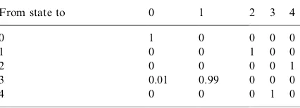
The four-attribute analysis yielded one cluster, suggesting that only one process is operating. The states within the cluster are summarised inTable 1 and the transition matrix is in Table 2. Fig. 1 illustrates the states and the main transitions between them.
Four of the states form a dynamic cycle of states of the form 1/2/4/3/1/2/4/3. . . with an occa-sional 3/0. Thus, as shown in Fig. 1, tall dense Sporobolus withvirtually noSarcocornia (State 1) changes to very sparse, short Sporobolus with sparse, very short Sarcocornia (State 2), which becomes very short, low densitySporobolus with sparse, large Sarcocornia (State 4), then very dense, moderate-sized Sarcocornia with virtually no Sporobolus (State 3) and then the pattern repeats. At the Sarcocornia state (3) only the change may be to bare ground (State 0) and, if so, it is a one-way path, i.e. State 0 is an absorbing state. The cyclic pattern may also reflect a second-order process, a possibility which will be discussed later. As for the effects of treatment, since there is only one cluster for all sites, irrespective of treatment, they all are contained within it and hence no significant effects of modification can be identified.
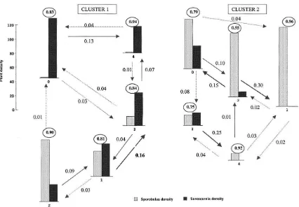
4.2. Two-attribute analysis: Sporobolus and Sarcocornia density
If only the density of the two species is examined we obtain two clusters or processes*/one essen-tiallySarcocornia (Cluster 1) and the other Spor-obolus (Cluster 2). The state descriptions and transition matrices are shown in Tables 3 and 4.
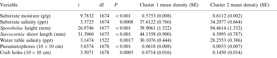
The t-test results, where significant, are shown in Table 5. The system is shown diagrammatically in Fig. 2.
The two processes appear to relate to the habitat characteristics of the two species. Cluster 1 ( Sar-cocornia) is drier, saltier, with shorterSporobolus and larger Sarcocornia, and it contains more mangrove pneumatophores than Cluster 2. Cluster 2 is wetter, less salty, has taller Sporobolus, very shortSarcocornia and has more crab holes. One of the local grapsid crab species (Parasesarma ery-throdactyl) appears to prefer the Sporobolus environment (Chapman et al., 1998). Each cluster or process differentiates the states within the species. Within each cluster there are five states which show similarvariations to those of the four-attribute process model. The states defined for one cluster appear to have little in common with those of the other. Cluster 1 shows clear diagonal dominance in the transition matrix (Table 4), with self-transitions ranging from 0.810 to 0.944, which indicates that the vegetation is stable. Cluster 2 also shows this tendency, though less markedly, except for State 2. The range of self-transitions is 0.547/0.955.
Table 1
The four-attribute analysis*/state descriptions
State Sporobolusmean density (SD)
Sporobolusmean height (mm) (SD)
Sarcocornia mean density (SD)
Sarcocorniamean size (mm) (SD)
0 0.001 (0.04) 0.052 (1.49) 0.005 (0.18) 0 (2.25)
1 127.948 (73.06) 97.55 (41.37) 0.044 (0.51) 0 (0)
2 0.626 (0.07) 33.572 (19.70) 6.583 (0.49) 0 (12.67)
3 0 (0) 0.12 (0.37) 92.078 (4.15) 16.76 (0.72)
4 28.318 (11.74) 2.00 (0) 2.578 (1.12) 66.111 (3.14)
Table 2
Transition matrix for the four-attribute analysis
From state to 0 1 2 3 4
0 1 0 0 0 0
1 0 0 1 0 0
2 0 0 0 0 1
3 0.01 0.99 0 0 0
There was no significant relationship between treatment and cluster. This again indicates that runnelling has not modified the processes operat-ing, even though the observed data are hetero-geneous.
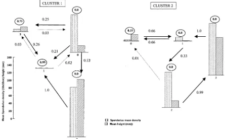
4.3. Two-attribute, one-species analysis: Sporobolus density and height
If we restrict the analysis to Sporobolus only, since it is more widespread thanSarcocorniaat the site, we again get two clusters each of four states. The state descriptions are in Table 6 and the transition matrices in Table 7. Fig. 3 shows the pattern of change graphically.
Neither cluster here shows the marked diagonal dominance of the transition matrices that ap-peared in the previous analysis. Cluster 2 is more dynamic than Cluster 1 with larger off-diagonal elements. In Cluster 1 all states may go to bare ground (State 1), and State 2 (tall dense Sporobo-lus) always does so. The bare ground and sparse states (1 and 3) are unlikely to change, and this is similar to the four-attribute analysis. The situation is consistent withDale and Dale (2002)and makes sense in the field. Low densities and height of Sporobolus seem to change towards bare ground. This occurs, but to a lesser extent, in Cluster 2 as well, where State 0 (very sparse, shortSporobolus), which has very similar emission probabilities to State 3 of Cluster 1, generally becomes shorter (or stays the same). The similar states of moderately dense, shortSporobolus states (State 0 in Cluster 1; State 2 in Cluster 2), although having similar emission probabilities, are each part of a different process. In Cluster 1, State 0 directly or indirectly ends up as bare ground, but this is not so in Cluster 2 where State 2 cycles through large variations in height and density but does not reach an empty state.
Fig. 1. Four-attribute data*/one cluster.
Table 3
State descriptions for the two-attribute, two-cluster result
State Cluster 1 Cluster 2
Sporobolusmean density (SD)
Sarcocorniamean density (SD)
Sporobolusmean density (SD)
Sarcocorniamean density (SD)
0 1.38 (4.03) 84.7 (44.2) 69.511 (35.88) 32.191 (18.39)
1 35.5 (13.4) 46.1 (27.9) 112.059 (58.67) 0 (0.06)
2 87.5 (28.3) 24.4 (18.2) 90.637 (37.146) 7.483 (4.89)
3 13.0 (7.9) 46.7 (29.9) 15.114 (12.37) 17.767 (15.10)
The environmental attributes with significantt -test results are shown inTable 8. Cluster 1, which is prone to reach the bare ground state, is drier, saltier and has more and largerSarcocornia than Cluster 2, indicating that this cluster is from a lower marsh position closer to the mangroves which fringe the marsh on the seaward edge (Adam et al., 1988). In support of this there was a significant relationship with distance from the flooding inlet, with Cluster 1 being considerably closer to it (Table 8). Again there was no significant relationship between the clusters and whether a site had been modified or not.
5. Discussion
5.1. Substantive results on the impact of runnelling
Overall, we find that there is no evidence that our treatment has modified the processes operat-ing to control thevegetation changes in the marsh. From other evidence (Dale et al., 1993, 1996; Dale, 2001) we have identified areas of the marsh which have changed after the treatment, generally be-coming wetter, but they apparently remain within the range of states of the system. As wetness has increased, the density ofSporobolus has decreased, Table 4
Transition matrices for the two-attribute (SporobolusandSarcocorniadensity) two-cluster result
From-state-to 0 1 2 3 4
Cluster1
0 0.832 0.002 0.000 0.034 0.13
1 0.000 0.810 0.027 0.163 0
2 0.009 0.090 0.902 0.000 0
3 0.037 0.040 0.005 0.844 0.07
4 0.042 0 0.003 0.011 0.944
Cluster2
0 0.789 0.040 0.099 0.082 0
1 0.002 0.955 0.023 0.002 0.018
2 0.149 0.303 0.547 0.001 0
3 0 0 0 0.752 0.248
4 0 0.034 0.007 0.036 0.923
Table 5
The two-attribute analysis:SporobolusandSarcocorniadensity and significant relationships with other attribute not used in the cluster analysis
Variable t df P Cluster 1 mean density (SE) Cluster 2 mean density (SE)
Substrate moisture (g/g) 9.7832 1674 B/0.001 0.5753 (0.008) 0.6112 (0.002)
Substrate salinity (ppt) 3.3725 1674 0.0008 37.6122 (0.760) 34.2077 (0.664) Sporobolusheight (mm) 26.9746 1677 B/0.001 39.9061 (1.522) 94.4614 (1.332)
Sarcocorniashoot length (mm) 31.3960 1675 B/0.001 44.1358 (0.900) 6.5995 (0.787)
Water table salinity (ppt) 3.1474 1522 0.0017 30.1076 (0.444) 28.2553 (0.386) Pneumatophores (10/10 cm) 5.6574 1678 B/0.001 0.0618 (0.008) 0.0053 (0.007)
since Sporobolus tends to be found in slightly higher areas (Adam et al., 1988). The increased wetness and reduced Sporobolus are associated also with increased crab activity (Chapman et al., 1998), but the causal mechanisms are not clear. Other results are consistent with what is known about the plants. Such results include:
. the inverse relationship in the distribution of Sporobolus andSarcocornia;
. the lower salinity environment ofSporobolus at greater distance from the tidal source; and . the increased presence of mangrove
pneumato-phores in areas of higher salinity, whereas crab activity is greatest in the wetter places.
Changes identified in the field and in remote sensing research are consistent with the findings here. ThusDale et al. (1996)identified a reduction inSporoboluscover and biomass in the study area Fig. 2. Two-attribute data*/SporobolusandSarcocorniadensity, two clusters (key as forFig. 1).
Table 6
State descriptions for the two-attribute, one species analysis ofSporobolusdensity and height
State Cluster 1 Cluster 2
Sporobolusmean density (SD) Sporobolusmean density (SD) Sporobolusmean density (SD) Sporobolusmean density (SD)
0 98.046 (2.59) 16.688 (0.69) 3.204 (2.59) 16.954 (50.75)
1 0.001 (0.50) 0.014 (0.494) 9.979 (15.51) 0.680 (0.94)
between 1983 and 1991, and the analysis in Dale and Dale (submitted for publication) clearly iden-tified an absorbing state which is bare ground. In the present analyses the four-attribute single process result with five states identified this, and to a lesser extent it appeared in Cluster 1 of the
two-attribute analysis of Sporobolus density and height. It was not apparent in the two-attribute Sporobolus andSarcocornia density analysis. This perhaps illustrates that the selection of attributes can have a marked effect on the results and their interpretation. The cyclic nature of the changes of state may be related to season or may reflect local effects of tides, which have a lunar cycle.
5.2. Methodological
Although there are many other ways of ev aluat-ing the similarity between series of observations (for example Merriam and Sneath, 1966; Lance and Williams, 1967; Dale et al., 1970; Juang and Rabiner, 1985;Little and Ross, 1985; Dale et al., 1988; Agrawal et al., 1995;Bollob’as et al., 1997; Allison, 1998; Oates et al., 1998; Edgoose and Allison, 1999; Perng et al., 2000), we shall con-centrate on the HMM approach, for which there remain several issues to consider. These include: Table 7
Transition matrices for the two-attribute, one species analysis ofSporobolusdensity and height
From state to 0 1 2 3
Cluster1
0 0 0.214 0.534 0.251
1 0.023 0.950 0 0.027
2 0 1.000 0 0
3 0.025 0.261 0 0.714
Cluster2
0 0.334 0.666 0 0
1 0.666 0 0.334 0
2 0.011 0 0 0.989
3 0 1.000 0 0
. data stability, coarseness andvariance;
. the propriety of using first-order Markov models, especially when nonlinearity, nonsta-tionarity and system memory are likely (Lee, 1990);
. the use of crisp clusters and its implication for consistency of estimates and model uncertainty; . the potential environmental interpretation of
states.
5.2.1. Data coarseness andvariance
Muchvegetation data are collected using coarse measures such as ordered categories. We should strictly introduce a trade-off between the coarse-ness of the specification of parameters and the loss of fit induced by crude estimates of parameters, so that our model reflects the crudeness of our observation (Zukerman et al., 2000).Wallace and Dowe (2000), using the minimum message length principle, obtained a trade-off between the costs of encodingvery precise parameter estimates and the loss of fit to the data resulting from using coarse estimates. Palusˆ (1996a) has examined this ques-tion in time series where continuous attributes have been quantised.
5.2.2. The suitability of Markovmodels
Markov models are relatively simple, though powerful, models, but they are certainly not the only possibilities for modelling sequences.Raftery and Tavare (1994), Liebovitch (1995), Stanley et
al. (1995), Le et al. (1996) have all proposed generalisations and alternatives. Ostendorf et al. (1966) discussed specific shortcomings of HMMs for continuous speech recognition, which is a problem akin to vegetation sequence studies.3 They specifically recognise the weak modelling of duration, the assumptions of conditional indepen-dence of observations given the state sequence, and the restrictions on feature extraction imposed by frame-based observations, which is really a question of scale.
Orlo´ci et al. (1993)have, in contrast, argued that a Markovmodel is suitable for studyingvegetation processes. However, theoretical considerations are probably overruled by practical considerations. In order to estimate parameters for more complex models we need long data sequences, and these are usually not available. The ‘memory’ of an ecolo-gical system might be quite long, and the collection of data over periods of time, which might reach centuries for forests, is simply infeasible.
5.2.3. Nonstationarity
We have assumed that the parameters of the models fitted to a group of sequences do not change with time; that is the estimates do not depend on where in the sequence we start. This assumption is unlikely to be true in ecological studies where responses to environmental changes may well mean that the parameters themselves vary. An example would be the effects of radiation reported byBall et al. (1991). Such nonstationarity is also intimately related to, and may be indis-tinguishable from, nonlinearity.
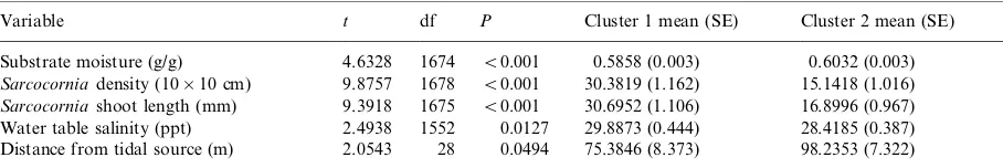
In the four-attribute results, the processes ap-peared to be operating in a cyclic manner. In this case the starting point in a sequence may not be Table 8
The two-attribute, one species analysis ofSporobolusdensity and height*/other significantly relatedvariables
Variable t df P Cluster 1 mean (SE) Cluster 2 mean (SE)
Substrate moisture (g/g) 4.6328 1674 B/0.001 0.5858 (0.003) 0.6032 (0.003)
Sarcocorniadensity (10/10 cm) 9.8757 1678 B/0.001 30.3819 (1.162) 15.1418 (1.016)
Sarcocorniashoot length (mm) 9.3918 1675 B/0.001 30.6952 (1.106) 16.8996 (0.967)
Water table salinity (ppt) 2.4938 1552 0.0127 29.8873 (0.444) 28.4185 (0.387) Distance from tidal source (m) 2.0543 28 0.0494 75.3846 (8.373) 98.2353 (7.322)
3
important. However, if the starting point is critical, one approach would be to look for simple nonstationary models (trends, periodicities) to represent the time-varying aspects of any sequence (seeCox, 1958; Palusˆ, 1996b; Le et al., 1996). We can then try to remove them instead of complicat-ing our models directly, by examincomplicat-ing residuals after the removal of any nonstationary effects. Incorporation is also possible; for example,Sun et al. (1994)discuss nonstationary models. We might also look to semi-continuous or discrete Markov processes, especially if it is sensible to group our observations into events or episodes (see, e.g., Dietterich and Michalski, 1985; Mannila and Toivonen, 1996).
An appearance of nonstationarity can also result from non-Gaussian error distributions or variation in thevariance of the error distribution through time. These might be studied through the use of entropy rates. Entropy measures the error that we have in determining our location in a state space. Entropy rate considers how this error changes with time and can be measured using the Kolmogorov/Sinai or metric entropy rate (Palusˆ, 1997). Entropy rate is the maximal diversity of patterns in a data stream and can be related to mutual information. Again, long sequences are necessary to investigate such maters.
A somewhat similar problem occurs when a single series of observations changes its generating process one, or more times, perhaps because of environmental fluctuation. A single model for the entire sequence is then inappropriate, although between such changes a simple model may be adequate. Change-point estimation has been the object of much study, as have been other aspects of within-sequence similarity and dissimilarity (see, e.g.,Lawrence et al., 1993).
5.2.4. Higher order processes
Due to the limited duration of observations, we have chosen to use first-order Markov processes only. This means that the next state of the system is dependent only on the present state, i.e. the system has no memory. Ecologically, this means that a snapshot of the vegetation at one time provides a reasonable basis for predicting its future state, which has considerable practical
significance. There is some evidence that this assumption is untrue in the ‘two-attribute one-species’ analysis. Here we have two clusters, but in each there exists a state with emission probabilities similar to a state in the other cluster. However, the transition probabilities differ for the two states. This does mean that observationally indistinguish-able sites could have different futures. How, then, is this future to be determined? While the emission probabilities are not exact descriptions of the hidden state, we do not have proof of higher order processes; this does suggest that memory is present in the system. We will attempt an assessment of the amount of memory in our system elsewhere. The four-attribute result may also reflect a second-order process describing some periodic changes using three states based on height alone: low, moderate and tall. Sporobolus and Sarcocornia seem to be negatively correlated and the model simply needs greater complexity to distinguish low0/moderate from tall0/moderate transitions.
To avoid the complexity of a second-order (or higher) model, we can transform it into a first-order model in the following way. In a second-order model the transition probabilities depend on the previous two states. We recode the pairs of states to produce ‘new’ states. Given a sequence 1/ 2/4/3/1/2/4/3. . ., we might recode 1/2 to W, 2/4 to X, 4/3 to Y, 3/1 to Z, which results in a (first-order) process WXYZWXYZ. . ., i.e. we code every pair of symbols using a new symbol, using overlapping pairs. By this means we obtain a first-order sequence, using W, X, Y and Z. Forn initial states we would finally haven2states, although not all of these may actually be observed. For a third-order process we would need to consider triples and hence up to n3 possible states. This simply trades the order of model against the number of states.
5.2.5. Partial assignment, model uncertainty and consistency of estimates
parameters. By allowing things to be probabilisti-cally (fuzzily) assigned to several clusters, this inconsistency can be removed. Such a procedure also incorporates model uncertainty, for ev ery-thing is effectively associated with the model of every cluster. Clusters of HMMs seem likely to behave similarly.
5.3. Environmental interpretation
Although we have here relied on simple tests, it is obvious that we could analyse the environmental data in the same HMM manner as the plant data, although perhaps the Gaussian assumption for emissions is less acceptable and other distributions would have to be introduced. We would then have a second set of HMMs that would form a basis for comparison of the two results.Juang and Rabiner (1985)have examined similarity measures between HMMs, so that inter-cluster relationships can be examined, while Allison et al. (1990) used ‘pair HMMs’ for a similar purpose.
In summary, in this paper we have shown how the use of HMMs allows us to identify the nature of a given treatment. In this particular case there is no evidence that runnelling introduces changes in the processes operating in the salt marsh, for a single HMM is sufficient to capture the temporal variation. We have also shown that restricting the descriptors to Sporobolus properties only shows that Sporobolus is acting in different ways in different parts of the marsh, though this hetero-geneity is not a reflection of our treatment. Instead, it probably reflects the relative position of a site on the marsh. Using the density of the two species as the only property we also obtain a different result, one which also identifies hetero-geneity in the system. This too may reflect position on the marsh. The brief analysis of the other environmental attributes does support these ideas in terms of wetness-related factors, which in turn are related to relative position on the marsh.
The biggest problem with this methodology, and with generalisations of it, is the need for the observations to be made over adequate periods of time. We have used 56 occasions representing 14 years of data collection, yet this is hardly sufficient even for first-order Markov processes. Extensions
to nonstationary, or other more complex, models would require much larger samples. What is clear is that using changes derived from observing two occasions cannot provide an acceptable assessment of the effects of impacts on the processes operating within a system and of its future course. Change in vegetation may be slow, but it is inexorable, and we accept predictions based on limited evidence at our peril.
Acknowledgements
We thank many student assistants who have helped to collect the field data over many years. We thank the Gold Coast City Council for providing boat transport to the study site for the whole time-period. Financial support has come from the Gold Coast City Council and the Mosquito and Arbovirus Research Committee, as well as from the Queensland State Health Department.
References
Adam, P., Wilson, N.C., Huntley, B., 1988. The phytosociology of coastal saltmarsh vegetation in New South Wales. Wetlands (Australia) 7, 35/84.
Agrawal, R., Lin, K.-I., Sawhney, H.S., Shim, K., 1995. Fast similarity search in the presence of noise, scaling and translation in time series databases. Proceedings of the 21st Very Large Database Conference, Zu¨rich, Switzerland. Akaike, H., 1978. A Bayesian analysis of the minimum AIC
procedure. Ann. Inst. Stat. Math. 30, 9/14.
Allison, L., 1998. Information-theoretic sequence alignment. Technical Report, 98/14, School of Computer Science, Monash University, Clayton, Victoria.
Allison, L., Wallace, C.S., Yee, C.N., 1990. Inductive inference over macro-molecules. Technical Report, 90/148, Depart-ment of Computer Science, Monash University, Clayton, Victoria.
Ball, M.C., Hodges, V.S., Laughlin, G.P., 1991. Cold-induced photoinhibition limits regeneration of snow gum at tree line. Funct. Ecol. 5, 663/668.
Banfield, J.D., Raftery, A.E., 1993. Model-based Gaussian and non-Gaussian clustering. Biometrics 49, 803/821. Bensmail, H., Celeux, G., Raftery, A.E., Roberts, C.P., 1995.
Bollob’as, B., Das, G., Gunopulos, D., Mannila, H., 1997. Time-series similarity problems and well-separated geo-metric sets. Available from:http://www.almaden.ibm.com/ cs/quest/papers/cg97_expanded.ps
Boulton, D.M., Wallace, C.S., 1970. A program for numerical classification. Comput. J. 13, 63/69.
Chapman, H., Dale, P.E.R., Kay, B.H., 1998. A method for assessing the effects of runnelling on salt-marsh grapsid crab populations. J. Am. Mosq. Control Assoc. 14, 61/68. Cox, D.R., 1958. The regression analysis of binary sequences. J.
R. Stat. Soc. Ser. B 20, 215/232.
Critchlow, D.E., 1980. Metric methods for analyzing partially ranked data. In: Lecture Notes in Statistics, vol. 34. Springer-Verlag, Berlin.
Dale, P.E.R., 2001. Wetlands of conservation significance: mosquito borne disease and its control. Arbovirus Res. Aust. 8, 102/108.
Dale, P.E.R., Dale, M.B., 2002. Optimal classification to describe environmental change: pictures from the exposi-tion. Community Ecol. 3, 19/29.
Dale, M.B., Macnaughton-Smith, P.W.T., Lance, G.N., 1970. Numerical classification of sequences. Aust. Comput. J. 2, 9/13.
Dale, M.B., Coutts, R., Dale, P.E.R., 1988. Landscape classification by sequences: a study of Toohey Forest. Vegetatio 29, 113/129.
Dale, P.E.R., Dale, P.T., Hulsman, K., Kay, B.H., 1993. Runnelling to control saltmarsh mosquitoes: long-term efficacy and environmental impacts. J. Am. Mosq. Control Assoc. 9, 174/181.
Dale, P.E.R., Chandica, A.L., Evans, M., 1996. Using image subtraction and classification to evaluate change in sub-tropical intertidal wetlands. Int. J. Remote Sensing 17, 703/ 719.
Dermatas, E., Kokkinakis, G., 1996. Algorithm for clustering continuous density hidden Markovmodel by recognition error. IEEE Trans. Speech Audio Process. 4, 231/234. Dietterich, T.G., Michalski, R.S., 1985. Discovering patterns in
sequences of events. Artif. Intell. 25, 287/332.
Edgoose, T., Allison, L., 1999. MML Markovclassification of sequential data. Stat. Comput. 9, 269/278.
Faith, D.P., Dostine, P.L., Humphrey, C.L., 1995. Detection of mining impacts on aquatic macroinvertebrate communities: results of a disturbance experiment and the design of a multivariate BACIP monitoring program at Coronation Hill, NT. Aust. J. Ecol. 20, 167/180.
Juang, B.H., Rabiner, L.R., 1985. A probabilistic distance measure for hidden Markov models. AT&T Tech. J. 64, 391/408.
Lance, G.N., Williams, W.T., 1967. Note on the classification of multilevel data. Comput. J. 9, 381/382.
Lawrence, C.E., Altschul, S.F., Boguski, M.S., Liu, J.S., Neuwald, A.F., Wootton, J.C., 1993. Detecting subtle sequence signals. Science 262, 208/214.
Le, N.D., Martin, R.D., Raftery, A.E., 1996. Modelling out-liers, bursts and flat stretches in time series using mixture
transition distribution (MTD) model. J. Am. Stat. Assoc. 91, 1504/1515.
Lee, K.F., 1990. Context-dependent phonetic hidden Markov
models for speaker independent continuous speech recogni-tion. IEEE Trans. Acoust. Speech Signal Process. 38, 599/ 609.
Li, C., Biswas, G., 1999. Temporal pattern generation using hidden Markovmodel-based unsupervised classification. In: Advances in Intelligent Data Analysis In: Lecture Notes in Computer Science, vol. 1642. Springer-Verlag, Berlin, pp. 245/256.
Li, C., Biswas, G., 2000. Bayesian temporal data clustering using hidden Markovmodel representation. In: Langley, P. (Ed.), Proceedings of the Seventeenth International Con-ference on Machine Learning. Morgan Kaufmann, San Francisco, CA, pp. 543/550.
Liebovitch, L.S., 1995. Ion channel kinetics. In: Iannaccane, P.M., Khokha, M.K. (Eds.), Fractal Geometry in Biological Systems: An Analytical Approach. CRC Press, London, pp. 31/56.
Little, I.P., Ross, D.R., 1985. The Levenshtein metric: a new means for soil classification tested by data from a sandpod-zol chronosequence and evaluated by discriminant analysis. Aust. J. Soil Res. 23, 115/130.
Mannila, H., Toivonen, H., 1996. Discovering generalized episodes using minimal occurrences. Proceedings of the Second International Conference on Knowledge Discovery and Data Mining (KDD’96), AAAI Press, Portland, OR, pp. 146/151.
Merriam, D.F., Sneath, P.H.A., 1966. Quantitative comparison of contour maps. J. Geophys. Res. 71, 1105/1115. Oates, T., Firoiu, L., Cohen, P.R., 1998. Clustering time series
with hidden Markov model and dynamic time warping. Proceedings of the 4th International Conference on Knowl-edge Discovery Datamining, New York, pp. 294/298. Orlo´ci, L., Anand, M., He, X.S., 1993. Markov chains: a
realistic model for temporal coenosere. Biom. Praxom. 33, 7/26.
Ostendorf, M., Digilakis, V., Kimball, O.A., 1966. From HMMs to segment models: a unified view of stochastic modelling for speech recognition. IEEE Trans. Speech Audio Process. 4, 360/378.
Palusˆ, M., 1996a. Coarse grained entropy rates for character-ization of complex time series. Physica D 93, 64/77. Palusˆ, M., 1996b. Detecting nonlinearity in multivariate time
series. Phys. Lett. A 213, 1387.
Palusˆ, M., 1997. Kolmogoroventropy from time series using information-theoretic functionals. Neural Netw. World 7, 269/292.
Perng, C.-S., Wang, H.-X., Zhang, S.R., Parker, D.S., 2000. Landmarks: a new model for similarity-based pattern querying in time series databases. Sixteenth International Conference on Data Engineering, pp. 33/47.
Raftery, A.E., Tavare, S., 1994. Estimation and modelling repeated patterns in high-order Markov chains with the mixture transition distribution (MTD) model. Appl. Stat. 4, 178/200.
Schwarz, G., 1978. Estimating dimension of a model. Ann. Stat. 6, 461/464.
Sebastiani, P., Ramoni, M., Cohen, P., Warwick, J., Davis, P., 1999. Discovering dynamics using Bayesian clustering. In: Proceedings of the 3rd International Symposium on In-telligent Data Analysis.
Smyth, P., 1997. Clustering sequences with hidden Markov
models. In: Mozer, M.C., Jordan, M.I., Petsche, T. (Eds.), Advanced Neural Information Process, vol. 9. MIT Press, Cambridge, MA.
Stanley, H.E., Buldyrev, S.V., Goldberger, A.L., Havlin, S., Mantegna, R.S., Peng, C.-K., Simons, M., 1995. Scale invariant features of coding and noncoding DNA
se-quences. In: Iannaccane, P.M., Khokha, M.K. (Eds.), Fractal Geometry in Biological Systems: An Analytical Approach. CRC Press, London, pp. 15/30.
Sun, D., Deng, L., Wu, C., 1994. State-dependent time warping in the trended hidden Markovmodel. Signal Process. 39, 263/275.
Wallace, C.S., Dowe, D.L., 2000. MML clustering of multi-state, Poisson, von Mises circular and Gaussian distribu-tions. Stat. Comput. 10, 73/83.
Wallace, C.S., Freeman, P.R., 1987. Estimation and inference by compact coding. J. R. Stat. Soc. B 49, 240/252. Zukerman, I., Albrecht, D.W., Nicholson, A.E., Doklo, K.,