Economics of Education Review 18 (1999) 89–105
The variation in teachers’ grading practices: causes and
consequences
Hans Bonesrønning
*Department of Economics, Norwegian University of Science and Technology, N-7055, Dragvoll, Norway Received 1 January 1997; accepted 8 January 1998
Abstract
The teachers’ grading practices vary a lot between the upper secondary schools in Norway. This paper discusses the causes and the consequences. The point of departure is the model laid out by Correa and Gruver (1987), which incorpor-ates grades as a policy instrument for the teacher who tries to manipulate the students’ studying time. However, in the Norwegian institutional setting students have incentives to press for easy grading. We therefore introduce an alternative grading model with rent seeking students, that is, students who allocate time to affect the teachers’ grading. We then provide empirical evidence that the teachers’ grading is systematically associated with teacher characteristics, and discuss whether this is consistent with the Correa and Gruver’s model, the alternative model or both. Thereafter the consequences of teachers’ grading for student achievement is investigated empirically. Our tentative interpretation of the results is that hard grading improves student achievement. [JELI21].1998 Elsevier Science Ltd. All rights reserved.
1. Introduction
This paper provides empirical evidence that teachers’ grading practices vary substantially between upper sec-ondary schools in Norway, and it sets out to investigate the causes and the consequences. The focus is on the potential incentive effects of teachers’ grading. The main hypothesis to be investigated is whether student achieve-ment is affected by the ways teachers reward students during the learning process. This is an important issue related to the current debate whether incentives-oriented school reforms will succeed or not.
The understanding of the incentives currently in place in schools may in fact be a necessary prerequisite for successful school reforms. Hoenack (1994) states that economists have underemphasized these topics in their analysis of education, and moreover, that very little attention has been given by academics to the question of incentives on students. We therefore expect the marginal returns to investigations of the students’ current incen-tives to be rather large.
* E-mail: [email protected]
0272-7757/98/$ - see front matter1998 Elsevier Science Ltd. All rights reserved. PII: S 0 2 7 2 - 7 7 5 7 ( 9 8 ) 0 0 0 1 2 - 0
Our point of departure is the student-teacher interac-tion model set out by Correa and Gruver (1987). This model applies the assumption that students care about perceived achievement, defined as the product of real achievement and a teacher’s grading parameter. The grading parameter is a potential control variable for the teacher trying to manipulate students, because it affects the opportunity cost of the time students allocate to other activities than education. The effect of a change in teach-er’s grading on a student’s allocation of time cannot be determined — unless rather strong assumptions are made about student preferences and the teaching technology. Montmarquette and Mahseredjian (1989) apply the Cor-rea and Gruver’s model for a sample of Canadian pri-mary school pupils and provide evidence that hard grad-ing, i.e. grades set below the real achievement level, deterioriates the standardized test results for French lang-uage.1 In the work reported here we apply the same
1 Farkas and Hotchkiss (1989) discuss many of the issues
model for a sample of Norwegian upper secondary school students, and by separating between income and substitution effects, we find that hard grading ( 5 the income effect) has positive effects on student achieve-ment. There are several reasons why these results should not be regarded as definitive.
First, an assumption applied by Correa and Gruver — and by us in the empirical work reported above — is that students passively accept the teachers’ grading. This assumption is restrictive. It seems (more?) likely that the students recognize that they can improve perceived achievement by allocating time to influence teacher grad-ing practices. We augment the Correa and Gruver’s model with rent seeking students, and show theoretically that when students put pressure on teachers for easy grading, the relationship between grading and student achievement will be mediated through the students’ time constraints.
The crucial question then is which of the two models outlined above we should repose most confidence in. This is an empirical question: We find that teachers’ grading is systematically associated with teacher charac-teristics and discuss whether this finding is consistent with the Correa and Gruver’s model, the alternative model, or both. It turns out that none of the models can be excluded on the basis of this discussion. Thereafter, we investigate which theory provides a superior expla-nation in a formal statistical sense. We find no support for the rent seeking hypothesis, which imply that the conceptualization of grading as a teacher’s instrument seems appropriate.
Second, it turns out that the effects of teachers’ grad-ing cannot be (empirically) revealed unless relevant mea-sures of teacher heterogeneity are included. Montmar-quette and Mahseredjian (1989) present an illustrative discussion of the problems of separating between teach-ing quality and gradteach-ing effects when teacher character-istics correlate poorly with student achievement. Now, teacher heterogeneity represents the achilles heel of edu-cation production function studies. It is well known that student achievement adjusted for student traits, varies a lot across teachers, but that purchased teacher character-istics (education, experience) cannot explain much of the variation in student achievement. To deal with this prob-lem this paper utilizes the teachers’ own exam results from the universities as an additional measure of teacher heterogeneity. Fortunately, the teachers’ own exam results turns out to be an important determinant of teacher effectiveness.
Third, student self-selection might obfuscate the true relationships. After one year, the students in the upper secondary school are sorted into mathematics, social studies or foreign language by interaction between a selection criterion which is the probability of getting admission to the university and an underlying distri-bution of abilities and preferences. An example is that
students who respond to hard grading by increasing their studying time, may find that their probabilities of getting admission to the university increases when the grading gets harder. Students with preferences for hard grading may consequently sort themselves into the subjects with the hardest grading. We investigate whether the teachers’ grading practices affect the students’ specialization choices, and subsequently, we make the appropriate con-trols for selectivity bias while estimating the education production functions.
The paper is organized as follows. The model is laid out in Section 2. Section 3 provides empirical specifi-cations. In Section 4 data and results are presented, while concluding remarks are offered in Section 5.
2. The Model
Our basic framework is the teacher-student interaction model presented by Correa and Gruver (1987).2 This
model is within the education production function tra-dition insofar it has an achievement production function embedded, but it is a much richer approach including behavior assumptions regarding the two central actors; teachers and students. The major issue is that teachers and students react to each other’s working strategies. The model highlights the problem that policies attempting to increase student achievement by increasing the allocation of teacher time to education may have little or even negative effect on achievement due to reallocation of time on the part of the student. Grading is introduced as an instrument by which the teacher can reduce input sub-stitutions.
We make two modifications of the basic framework. First, Correa and Gruver apply the assumption that stu-dents care aboutperceivedachievement, which is defined as the product of real achievement and teacher grading. Teacher grading then is like a wage increase in a labor supply model. It produces counteracting income and sub-stitution effects, which are troubling in empirical work. We therefore introduce an alternative teacher grading model where the income and substitution effects are for-mally separated.3
Second, Correa and Gruver treat teacher grading as a policy variable by which the teacher can manipulate students’ studying time. This assumption may be too restrictive. Bishop (1989) has focused on how students establish peer pressure against studying hard when there
2The first contribution in the literature discussing incentives
on students which we are aware of, is Brown and Saks (1980), who introduce a model incorporating many of the same elements as Correa and Gruver.
3The separation between substitution and income effects is
is a lack of external standards for judging academic achievement. According to Bishop, this is part of the explanation for the apathy experienced in U.S. high schools. The institutional setting of the Norwegian upper secondary school is somewhat different. Admission to the university is decided on the basis of a mix of real and perceived achievement, which implies that students have to care about both components of achievement. In this setting it seems likely that students put pressure on teachers for easy grading, i.e. grades set above the real achievement level. Inspired by Bishop, we therefore aug-ment the Correa and Gruver’s model with rent seeking students. Student rent seeking may take many forms; we specify it as a time consuming activity. Examples are that students use some of their time in the classroom being non-cooperative if they receive too hard a grading. Successful rent seeking activities take grading away from the level preferred by the teacher. The grading level pre-ferred by the teacher is assumed to be equal to the grad-ing level preferred by the school principal. The rationale for this assumption is that a principal facing many teach-ers prefers consistent grading practices across classrooms, due to both equity and efficiency consider-ations. To achieve this goal the principal introduces (non-pecuniary )costs for the teachers who set grades that diverge from the principal’s preferred grading.
The Correa and Gruver’s model augmented with a modified relationship between perceived and real achievement and with rent seeking students is given by the following equations:
Eq. (1) is an achievement production function where student achievementvis assumed to be a concave func-tion of a student’s studying timeeand a teacher’s teach-ing timea. Different educational methods and qualitative characteristics of the teacher and the student can be rep-resented by different functional forms or by different values of the parameters. Byteaching qualitywe under-stand the stock of teacher characteristics (innate abilities, education, experience, the stock of teaching technologies) that is positively associated with student achievement, net of teacher teaching time and net of the teacher’s grading practices.
Eq. (2) says that student utility us is an increasing
function of student time to other activities osand
per-ceived achievementws. The student derives utility from
perceived achievement because it is one of the two pri-mary determinants of admission to a university and to a field of study. The marginal rate of substitution between ws and os reflects the achievement orientiation of the
student.
Eq. (3) portrays the teachers’ grading policy in the Norwegian upper secondary school. In Norway the tea-cher’s grades as well as the grades from the nationally administred exams are given on a 0–6 scale, where 0 and 1 represent failure and 6 is the best result. In Eq. (3)G3
is the teacher’s grade given a student who gets 3 on the external exam.G3describes the teacher as an easy grader
(G3> 3) or an hard grader (G3 ,3). gs describes the
degree to which the teacher’s grades vary with real achievement as measured by the external exam.
Eq. (4) says thatG3is a weighted sum of the student
rent seeking function G(r), and the grading level pre-ferred by the school principalGT. The rent seeking
func-tion is a concave funcfunc-tion of student rent seeking time r. The exact functional form of G(r) is determined by teacher and student characteristics. We assume that the teacher sets grades equal to the grades preferred by the school principal, GT, when students allocate no time to
rent seeking.areflects the cost to the teacher of deviat-ing from the principal’s preferred graddeviat-ing.a 50 implies that there are no such costs, whilea 5 1 implies that these costs are prohibitive large. The teacher’s grading practice is thus the result of student pressure for easy grading, the teacher’s ability to withstand pressure for easy grading, and the teacher’s costs of deviating from the principal’s preferred grading practices. By teacher strength we understand the teacher characteristics that shift the rent seeking function.
The assumption underlying Eq. (4) is that students influence the income effect (G3), but not the substitution
effect (gs). This restrictive model is rich enough to
illus-trate the new mechanisms that are introduced by rent seeking students. In the empirical part of the paper we also investigate whethergsis a function of student rent
seeking.
Eq. (5) is the student’s time constraint whereksis total
available time, and the other variables are defined above. Eqs. (6) and (7) are the teacher’s utility function and time constraint respectively.gT is the evaluation of the
teacher made by the school principal, and should be interpreted as the school principal’s instrument to affect the teacher’s teaching time. oT is the teacher’s time to
other activities. The marginal rate of substitution betweengTvand oTreflects the academic orientation of
the teacher.
consider the case without rent seeking students. That is, the Correa and Gruver’s assumption of exogenous grad-ing instruments applies.
In this case, and under the assumption that the teacher has set his/her teaching time equal toa5a9, the rational utility maximizing student chooses leisure and studying time according to Eq. (8).
uos9/uws9 5gsve9 (8)
Eq. (8) reads that the marginal increase in perceived achievement with respect to studying time is equal to the ratio of marginal utilities.
If the marginal returns to the external exam grades rises (gs↑), and G3 is adjusted to keep the utility level
unchanged, the student’s response will be to allocate more time to studying and less time to other activities (the substitution effect). If the teacher shifts from hard to easy grading (G3↑), the student’s response will be to
allocate less time to studying and more time to other activities in the case when leisure is a normal good, and more time to studying and less time to other activities in the case when leisure is an inferior good. Unfortunately, students’ attitude towards leisure may be an important dimension of student heterogeneity. The restrictive model then does not provide clearcut hypotheses about the relationship betweenG3and student achievement.
Next, assuming rent seeking students, the optimality conditions are:
uos9/uws5gsve9 5G9(r)(12a) (9)
The equality to the right says that in optimum an extra hour should yield the same increment in perceived achievement no matter if it is spent on studying or rent seeking.
If the teacher rises the marginal returns to the external exam grades (gs↑), the student’s response will be to use
more of his/her time for studying relative to rent seeking. Thus we expect (as above) thatgsis positively correlated
with real student achievement as measured by the exter-nal grades. If the teacher’s costs of deviating from the principal’s preferred grading increases (a↑), the marginal returns to rent seeking decrease and the student will real-locate his/her time towards studying time and time to other activities. It turns out that students with “high” elasticities of substitution between achievement and time to other activities in their utility functions respond to an increase in aby allocating more time to studying. An increase inais analogous to increased teacher strength. Appendix B provides a formal mathematical analysis for the special case of CES utility and achievement pro-duction functions.
One additional observation from the model is that low achieving students face the largest opportunities for rent seeking. To see this, note that neitherws norv can be
larger than 6. Assuming for simplicity thatgs5 1, we
have from Eq. (3)
ws5G31v23#6 (10)
A high achieving student experiencesv-values close to 6, while a low achieving student experiencesv-values far below 6. Eq. (10) then implies that the opportunity set for G3 is much larger for low achievers than for
high achievers.
This does not necessarily imply that low achieving students use more time for rent seeking than high achiev-ing students. The crucial question of course is whether the low achieving students also face the strongest incen-tives for rent seeking. The answer is that they might do, if they face smaller marginal returns to studying time than high achieving students.
So far we have focused on the grading issues. Some comments on the other elements of student-teacher inter-action are warrented.
From the first order conditions of the student’s maxim-ation problem we can define the student’s reaction func-tions
e*5f(a9,gs,GT,bs,bv,bg) (11)
r*5g(a9,gs,GT,bs,bv,bg) (12)
wherea9is the teaching time set by the teacher,gsis the
degree to which a teacher’s grades vary with achieve-ment,GTis the grading practices preferred by the school
principal andbi,i5s,v,g, represent the characteristics of
the student’s utility function, the achievement production function and the rent seeking function respectively. Some of the comparative static issues are discussed in Appendix B.
From the first order conditions of the teacher’s maxim-ation problem we can define the teacher’s reaction func-tion
a*5h(e9,gT,bv,buT) (13)
wherebuT represents the characteristics of the teacher’s
utility function and the other variables are explained above.
It is clear that the teaching time assumed by the stud-ent (a9) may differ from the equilibrium teaching time (a*), and no adjustment mechanisms are modelled.
Cor-rea and Gruver pay much attention to the game theoreti-cal equilibrium of teacher-student interaction. We realize that the problems of statistically analysing the model becomes much more complex when the game theoretical equilibrium is considered, but do not elaborate upon these issues here.
the students in the Norwegian upper secondary school have to choose which of the specialization subjects — mathematics, social studies or foreign language — they will study for the last two years in the upper secondary school. It seems likely that the demand for specialization subjects is determined by the expected pecuniary and non-pecuniary returns in interaction with abilities, tastes and some other factors. The teachers’ grading practices may affect the expected returns, for instance by affecting the probabilities of getting admission to the universities. When the teachers practice hard grading, some students may find that their probability of getting admission to higher education decreases, while other students may find that their admission probability increases. That is, the students may sort themselves across subjects depen-dent on their own abilities and preferences. An example is that the students who choose mathematics given hard grading, may be those students who respond to hard grading by allocating more time to studying. Thus, even if there exists no relationship between grading and stud-ent achievemstud-ent for all studstud-ents, such relationships may be revealed for mathematics due to sorting.
3. Empirical Specifications
Empirical specification of the modified Correa and Gruver’s model confronts the following problems: Neither students’ studying time, rent seeking time nor teachers’ teaching time are observable (without prohibi-tive costs) and besides, the grading parameters are latent variables. Thus the Eqs. (11)–(13) cannot be estimated directly. Inspired by Montmarquette and Mahseredjian (1989) we propose the following solutions.
Students’ academic achievement depends on optimal levels ofe*anda*. These optimal levels of studying time
and teaching time are interactive and depend on the characteristics of the achievement function, the charac-teristics of the student’s utility function, the character-istics of the rent seeking function, the charactercharacter-istics of the teacher’s utility function and the grading parameters GT and gT. A reduced form of the achievement
pro-duction function will thus link student achievement with these characteristics and the grading parameters. We have no data forGTand gT; these parameters are
there-fore assumed equal to 3 and 1 respectively. Then we have a standard education production function
vij5a01a1Xij1a2Yj1a3Zj1a4Xj1eij (14)
wherevijis the exam results for studentiin schoolj,Xij
is a vector of individual student characteristics for stud-entiin schoolj,Yjis a vector of teacher characteristics
for schoolj,Zjis a vector of school characteristics for
schoolj,Xjis a vector of student body characteristics for
school j and eij is an error term with standard nice
properties.
The inclusion of the Xij and Yj variables should be
clear from above. The elements in the Zj vector are
included as determinants ofa, and may also be seen as control variables capturing potential scale effects.Xj
cap-tures potential peer group effects and are included rather ad hoc.
We would like to separate the teacher characteristics associated with teaching quality from those associated with teacher strength. We are unable to do this a priori. The grading equation presented below may provide the information necessary to make the empirical separation between teaching quality and teacher strength possible.
Teacher grading depends on rent seeking time r*,
teacher strength, the costs of deviating from the grading parameter set by the principal and the grading preferred by the principal. In Section 2 we have argued that rent seeking time is associated with student characteristics. Consequently, we estimate the equation
G3
j 5b01b1Xj1b2Yj1b3Zj1mj (15)
whereG3
jis the grading parameter for schoolj,mjis an
error term, and the other variables are defined above. An indication that rent seeking actually occurs, will be that strong pressure for easy grading is associated with low achieving students. Unfortunately, we cannot reject the Correa and Gruver’s grading model on the basis of such findings, since significant relationships between grading and student (and teacher) characteristics may as well reflect that teachers are less than fully infor-med and that they conjecture that easy grading is “cor-rect” for low achievers.
The information provided by the estimation of Eq. (15) can be used to separate between teaching quality and grading effects/teacher strength effects in the esti-mation of the education production function. First, departing from the rent seeking interpretation, a two stage procedure where the predicted grading from Eq. (15) is used as an independent variable in Eq. (14), is appropriate. Second, departing from the policy instru-ment interpretation, the grading parameter should we treated as an exogenous variable and included directly in Eq. (14).
The remaining problem is how to measureG3andgs.
We propose the following relationship
wij 5G3j 1gjs(vij 23)1nij (16)
whereG3
jis the measure of teachers’ grading in school
j,gs
jdescribes the degree to which the teachers’ grades
vary with achievement as measured by the external exam between schools,vijis the external exam result for
stud-entiin schooljandnijis a random effect with standard
nice properties.
grades, the equation would be misspecified. Eq. (14) should instead be thought of as a definitional relationship that provides a measure of the divergence between exam results and teachers’ grades for each school.
To deal with the problem that students sort themselves into the specialization subjects, we apply the standard Heckman (1979) procedure. That is, the probability that a student chooses mathematics is estimated from a probit equation. The inverse Mill’s ratio is calculated from the probit equation and thereafter included in the education production function to correct for selectivity bias.
4. Data and Results
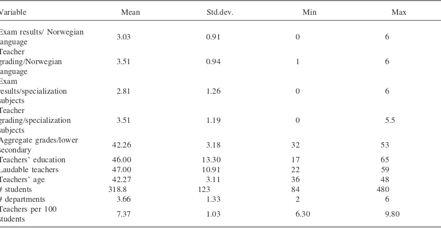
The analysis is based on a sample of 1092 academic students from 15 upper secondary schools in one Norwegian county. All students taking their final exam in 1990 are included. Table 1 presents the sample means and the standard deviations of the variables used in this study. Appendix A provides variable definitions. The teachers’ grades as well as the grades from the nationally administred exams are given on a 0–6 scale, where 0 and 1 represent failure and 6 is the best result. The table reports the teachers’ grades and the exam results for Norwegian language and the specialization subjects (mathematics, social sciences or foreign language). As can be seen, the teachers’ grades are set well above the exam results, indicating that the latent variable G3 is
larger than 3, or alternatively, that the latent variablegs
is larger than 1. The students’ initial level of knowledge
Table 1
Data means and standard deviations
Variable Mean Std.dev. Min Max
Exam results/ Norwegian
3.03 0.91 0 6
language Teacher
grading/Norwegian 3.51 0.94 1 6
language Exam
results/specialization 2.81 1.26 0 6
subjects Teacher
grading/specialization 3.51 1.19 0 5.5
subjects
Aggregate grades/lower
42.26 3.18 32 53
secondary
Teachers’ education 46.00 13.30 17 65
Laudable teachers 47.00 10.91 22 59
Teachers’ age 42.27 3.11 36 48
# students 318.8 123 84 480
# departments 3.66 1.33 2 6
Teachers per 100
7.37 1.03 6.30 9.80
students
is measured by an aggregate of their grades from the lower secondary school. 11 subjects are included, and the scale is 0–5. The variation in the average initial level of knowledge across schools basically reflects that some schools are in excess demand while others are in excess supply.
The teachers are characterized by experience, edu-cation and laudability. The two former characteristics are the conventional indicators for teacher quality in edu-cation production function studies, while teacher lauda-bility has not been utilized in any analysis we are aware of. The teachers’ teaching experience (school averages) varies between 10 and 20 years approximately. The tea-chers’ education is measured by the fraction of teachers having a master’s degree, i.e. we have essentially separ-ated between teachers with 4 and 6 years of education beyond secondary school. As can be seen, 47 percent of the teachers have laudable results from the universities and the variation between the schools is substantial.
Three school characteristics are reported; the number of teachers per 100 students, the number of students in the academic department and the total number of depart-ments within the school. The separation between the number of students within the academic department and the number of departments carries over from Bonesrøn-ning (1996), and reflects the upper secondary school organization with academic and vocational departments side by side.
stu-dents’ socioeconomic background simultanously influ-ence the students’ initial level of knowledge and their final achievement. We therefore expect the coefficient for the initial level of knowledge to be biased upwards. We do not expect that the other independent variables will be seriously affected by the omission of socioecon-omic background variables. This expectation is sup-ported by Hanushek and Taylor (1990), who provide evi-dence that serious misspecification problems are likely to be avoided when the students’ initial level of knowl-edge is included.
4.1. MeasuringG3andgs
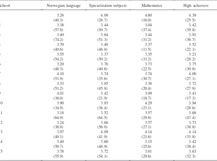
We have estimated Eq. (16) for the Norwegian langu-age, the specialization subjects and mathematics. The results are reported in Tables 2 and 3. As can be seen from Table 2, the estimatedG3
jcoefficients are above 3
without exception, and all G3
j are sharply determined.
The t-statistics are in the ranges above 16.0, which indi-cate that the coefficients are significantly different from zero at the 0.5 percent level. However, the t-statistics
Table 2
The grading parameter G3.t-statistics in parentheses
School Norwegian language Specialization subjects Mathematics High achievers
1 3.26 4.08 4.60 4.38
(40.3) (26.7) (16.0) (25.5)
2 3.38 3.44 3.04 3.42
(57.8) (50.7) (37.4) (39.8)
3 3.40 3.64 3.44 3.91
(74.2) (51.3) (31.2) (36.7)
4 3.70 3.40 3.37 3.52
(40.6) (46.8) (11.5) (22.1)
5 3.55 3.37 3.35 3.21
(54.2) (50.2) (33.2) (28.2)
6 3.20 3.76 3.73 3.75
(46.3) (40.6) (22.5) (30.8)
7 4.10 3.74 3.74 4.00
(51.9) (35.6) (30.7) (27.1)
8 3.33 3.85 3.38 3.72
(51.2) (45.8) (20.4) (27.9)
9 4.01 3.42 3.09 3.41
(36.0) (21.9) (18.7) (17.3)
10 3.90 3.93 4.29 3.94
(34.9) (36.4) (23.1) (28.6)
11 3.18 3.52 3.57 3.68
(64.9) (64.5) (29.8) (47.4)
12 3.24 3.66 3.57 3.73
(36.8) (56.0) (27.1) (38.8)
13 3.97 4.09 4.14 4.14
(40.1) (41.9) (21.6) (31.8)
14 3.40 3.60 3.15 3.42
(50.7) (46.9) (25.6) (38.4)
15 3.78 3.72 3.81 3.63
(55.9) (54.1) (29.6) (32.3)
give irrelevant information in this case. We therefore tested the equality of school means. The null hypothesis of the equality of school means is rejected for all sub-jects. Note that across subjects, mathematics shows the largest variation inG3
j. A student who gets the grade 3
on the external mathematics exam has the expected tea-chers’ grades 4.6 and 3.1 in the schools with the easiest and hardest grading respectively. This is somewhat sur-prising, since we intuitively think of mathematics as rather objective, with little leeway for teachers to evalu-ate equal achievements differently.
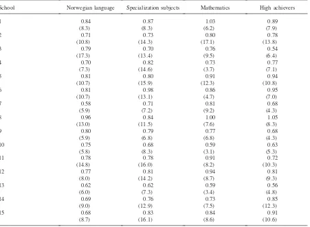
The estimatedgs
jare below 1 with a few exceptions.
The partial correlations betweenG3
jandgsjare negative
but rather small for all subjects, implying that the teach-ers’ grades vary less with achievement when the teachers practice easy grading. The partial correlation coefficient is very small in absolute value (0.03) for mathematics.
Table 3
The grading parameter gst-statistics in parentheses
School Norwegian language Specialization subjects Mathematics High achievers
1 0.84 0.87 1.03 0.89
(8.3) (8.3) (6.2) (7.9)
2 0.71 0.73 0.80 0.78
(10.8) (14.3) (17.1) (13.8)
3 0.79 0.70 0.76 0.54
(17.3) (13.4) (9.5) (6.4)
4 0.70 0.82 0.73 0.77
(7.3) (14.6) (3.7) (7.1)
5 0.81 0.80 0.91 0.94
(10.7) (15.9) (12.3) (10.8)
6 0.81 0.98 0.86 0.95
(10.7) (13.1) (4.7) (7.0)
7 0.58 0.71 0.81 0.68
(5.9) (7.2) (9.2) (4.3)
8 0.96 0.84 1.00 1.05
(13.0) (11.5) (7.6) (8.3)
9 0.80 0.79 0.77 0.68
(5.9) (6.8) (6.8) (4.3)
10 0.75 0.68 0.59 0.63
(5.8) (8.3) (3.1) (5.3)
11 0.78 0.78 0.91 0.72
(14.8) (16.0) (8.2) (10.3)
12 0.77 0.81 0.94 0.81
(8.0) (14.2) (8.7) (9.3)
13 0.62 0.62 0.59 0.56
(6.0) (7.3) (3.4) (4.8)
14 0.69 0.76 0.73 0.85
(9.0) (12.9) (7.5) (12.3)
15 0.68 0.83 0.84 0.91
(8.7) (16.1) (8.6) (10.6)
teacher and student characteristics, and further, how the grading practices are related to student achievement. We start the investigation of these questions by estimating the standard education production function. This is the correct reduced form when grading is endogenous, and it serves as our benchmark model.
4.2. The Standard Education Production Function
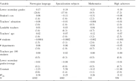
The estimation of Eq. (14) for the Norwegian langu-age, for the specialization subjects, for mathematics and for high achievers in the specialization subjects are reported in Table 4.
Table 4 confirms three important previous findings from education production function studies. First, the best predictor of individual students’ achievement is their initial level of knowledge, and the coefficient is very sharply determined. Note however that since no socioeconomic variables are included, the estimated coefficient for the initial level of knowledge is most likely biased upwards. Second, the number of teachers per student does not seem to influence student
achieve-ment. We have been careful in specifying the teacher input exclusive all extra classroom activities, but have been restricted to treat the teacher input as a school spe-cific variable. The latter is a problem if for instance low achievers are assigned to smaller classes, but the student allocation to different class sizes is very much a random process in the academic departments included in this study. It remains of course that if measurement error exists, the estimated coefficient of the teacher-student ratio will be biased towards zero. Our third finding con-sistent with earlier studies is that more educated teachers will not improve upon student achievement. One interpretation of the results is that simple accumulation of credits with no regard for the subjects being taught has no positive effect on student achievement. However, the significant negative sign of some of the estimated teachers’ education coefficients remains a puzzle.
Table 4
The standard education production functiont-statistics in parentheses
Variable Norwegian language Specialization subjects Mathematics High achievers
Lower secondary grades 0.17 0.19 0.21 0.19
(24.6) (17.8) (8.5) (7.2)
Student’s sex 0.06 20.11 20.31 20.08
(1.4) (1.6) (2.2) (0.8)
Teachers’ education 20.08 20.01 20.004 20.01
(3.0) (1.8) (0.5) (1.0)
Laudable teachers 0.01 0.03 0.04 0.03
(3.4) (6.3) (4.7) (4.1)
Teachers’ age 0.02 0.07 0.12 0.07
(1.6) (3.8) (3.2) (2.5)
# students 20.0004 20.0002 20.002 20.001
(1.5) (3.1) (2.8) (1.5)
# departments 0.06 0.06 0.04 20.05
(3.0) (1.9) (0.7) (1.2)
Teachers per 100
0.00 0.02 0.00 0.00
students
(0.5) (0.3) (0.5) (0.8)
Lower secondary
20.01 20.08 20.01 20.01
grades/average
(0.1) (0.8) (0.5) (0.7)
Constant 22.23 5.58 28.12 211.88
(0.8) (1.4) (1.1) (2.0)
R2
adj 0.38 0.25 0.26 0.12
N 1092 1092 332 559
relationship of the expected positive sign, while 7 dis-play a statistically negative relationship. 69 studies are not significant at the 5 percent level. Our analysis shows that teacher experience has a significant and positive influence on student achievement in all the reported specifications. Teacher experience seems to matter least in Norwegian language and most in mathematics. In mathematics, the difference between the school with the least experienced and the most experienced teachers is 1.44 grades, all else equal. Since this is a substantial effect, we should try to sort out the reasons why experi-ence show a strong positive association with student achievement in this study.
First, the positive correlation may result from more senior teachers having the ability to select schools and classrooms with better students. This possibility is men-tioned by Hanushek (1986). We have investigated whether teacher experience is associated with school and community characteristics, but it turns out that no stat-istically significant relationships exist.4
4In Bonesrønning (1996), where the relationship between
school size and student achievement is investigated empirically, I find evidence that the teacher input is endogenous. The sample used in this paper is a subsample of the sample used in Bonesrønning (1996). Thus, teacher behavior may differ between the Norwegian counties.
Second, we have tested the hypothesis that there exists an optimal number of teaching years, but the hypothesis has been rejected. Recall that teachers’ experience varies little across the schools in our sample. This variation may very well be within a relative linear part of a con-cave relationship. Further investigations are needed to settle this question.5
Third, the importance of teacher experience may have been obfuscated in previous analyses due to omitted vari-ables. We have estimated, but not reported, Eq. (14) without the fraction of laudable teachers included. It turns out that the significant association between teacher experience and student achievement disappears when the laudability variable is excluded. For this sample at least, the importance of purchased teacher characteristics is revealed only when appropriate controls are made for relevant non-purchased teacher characteristics.
The “new” indicator, the fraction of laudable teachers
5Many of the students from the 68-generation became
to all teachers, shows a significant and positive associ-ation with student achievement in all specificassoci-ations reported in Table 4. In mathematics, the difference in student achievement between the schools with the lowest and the highest fractions of laudable teachers is 1.48 grades, all else equal. The positive association between laudability and student achievement is an intuitive plaus-ible result, since laudability indicates that the teachers have good understanding of the subjects they teach. Note however that the theoretical analysis has focused on two mechanisms —teaching quality and teacher strength — through which teachers can influence student achieve-ment. We are of course unable to separate between the influences from these two factors on the basis of the results in Table 4, but will return to this issue below.
Now we investigate the relationships between grading practices and teacher characteristics.
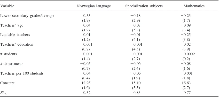
4.3. The Grading Equation
Eq. (15) is estimated by ordinary least squares with G3as the dependent variable. The results are reported in
Table 5. As can be seen, the grading in Norwegian lang-uage is not significantly associated with any of the teacher characteristics, while the grading in the speciali-zation subjects and mathematics is strongly correlated with all the teacher characteristics. For the latter subjects, it is evident that laudable and experienced teachers tice hard grading, while the most educated teachers prac-tice easy grading. Moreover, in the specialization sub-jects and mathematics the grading parameter is negatively associated with the students’ average initial level of knowledge. The null hypothesis that the
teach-Table 5
The grading equation. Dependent variable G3, t-statistics in parentheses
Variable Norwegian language Specialization subjects Mathematics
Lower secondary grades/average 0.33 20.18 20.23
(1.9) (2.9) (1.7)
Teachers’ age 0.04 20.07 20.09
(1.2) (5.7) (3.4)
Laudable teachers 0.01 20.01 20.25
(1.2) (4.1) (3.8)
Teachers’ education 0.001 0.001 0.02
(0.2) (4.5) (3.9)
# students 20.001 0.001 0.0002
(1.4) (2.7) (0.2)
# departments 20.05 20.06 20.08
(0.7) (2.4) (1.6)
Teachers per 100 students 0.04 20.06 0.001
(0.4) (1.9) (1.8)
Constant 212.26 15.10 16.63
(1.6) (5.5) (2.7)
R2
adj 0.32 0.83 0.77
ers’ grading practices are not affected by the students’ average initial level of knowledge is formally rejected for the specialization subjects, but not for mathematics. Note that we have not corrected for the multilevel character of the data involved in this analysis. In general, such correction implies more conservative estimates.
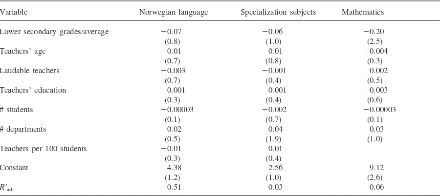
Table 6 reports the OLS-estimation results withgs jas
the dependent variable. There is basically no evidence that the degree to which the teachers’ grades vary with achievement correlates with teacher characteristics.
Note that Table 5, columns (2) and (3), provide evi-dence that the teacher characteristics are associated with hard grading in a way very similar to the association between teacher characteristics and student achievement in Table 4. The crucial question then is whether these teacher characteristics affect student achievement directly, or whether the teachers’ influence on student achievement is mediated through the grading practices. This issue is now investigated within the education pro-duction function framework.
Table 6
The grading equation. Dependent variable gs, t-statistics in parentheses
Variable Norwegian language Specialization subjects Mathematics
Lower secondary grades/average 20.07 20.06 20.20
(0.8) (1.0) (2.5)
Teachers’ age 20.01 0.01 20.004
(0.7) (0.8) (0.3)
Laudable teachers 20.003 20.001 0.002
(0.7) (0.4) (0.5)
Teachers’ education 0.001 0.001 20.003
(0.3) (0.4) (0.6)
# students 20.00003 20.002 20.00003
(0.1) (0.7) (0.1)
# departments 0.02 0.04 0.03
(0.5) (1.9) (1.0)
Teachers per 100 students 20.01 0.01
(0.3) (0.4)
Constant 4.38 2.56 9.12
(1.2) (1.0) (2.6)
R2
adj 20.51 20.03 0.06
low achievers are less capable of affecting grading when the fraction of laudable teachers increases. These results are consistent the model predictions: With increasing teacher strength, the rent seeking frontier shifts inwards, which implies that the marginal returns to student rent seeking decreases.
However, the results may as well be interpreted as showing i) that laudable and experienced teachers know more about grading than other teachers (admittedly, this interpretation take into account empirical results not presented yet), and ii) that all types of teachers conjec-ture that it is efficient to practice easy grading for low achievers.
These interpretations motivate two different approaches to the education production function, to be presented below.
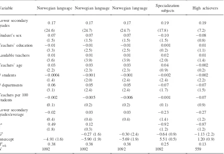
4.4. The Education Production Function Revisited (I)
We start with the interpretation that grading is a policy instrument for the teacher. Thus grading should be regarded as an exogenous variable to be included in the education production function.
Table 7 reports the results from estimation of the edu-cation producton function augmented with the grading parametersG3and gs. For Norwegian language, G3and
gsare both significantly associated with student
achieve-ment when included one at a time, while neither of the grading parameters turn out to be significant predictors of student achievement when included simultanously in the equation. The signs of the coefficients indicate that students i) respond to harder grading by increasing their studying time and ii) respond to increased marginal
returns to achievement by increasing their studying time. The magnitude of the grading effect (the G3 effect) is
illustrated by the following example. A student in the school who practice the hardest grading performs 0.28 grades better than a student in the school which practice the easiest grading, all else equal.
The G3 coefficient is not significant different from
zero for the specialization subjects, but when restricted to the sample of high achieving students, the G3
coef-ficient turns out to be a significant predictor of student achievement. The negative sign indicates that high achieving students treat leisure as a normal good. More-over, the grading effect is substantial. The sample vari-ation in G3 multiplied by the estimated coefficient is
equal to 1.3 grades. Thegscoefficient is not significantly
associated with student achievement, but the sign of the gscoefficient indicates that students allocate less time to
studying when the marginal returns to real achievement increases. Since thegseffect should be interpreted as a
substitution effect, this is a puzzling result. It might indi-cate that our estimation strategy of treating the speciali-zation subjects as one subject is inappropriate.
To mitigate these problems we highlight mathematics which is one of the specialization subjects. We consider the self-selection issue by estimating a selection equation with the dependent variable equal to 1 if the student choose mathematics and 0 otherwise. The independent variables are individual student characteristics and two grading parameters which are the G3 parameters for
mathematics and for all the specialization subjects net of mathematics. The results are reported in Table 8, col-umn (1).
math-Table 7
The education production function revisited (I)t-statistics in parentheses
Specialization
Variable Norwegian language Norwegian language Norwegian language High achievers subjects
Lower secondary
0.17 0.17 0.17 0.19 0.19
grades
(24.6) (24.7) (24.7) (17.8) (7.2)
Student’s sex 0.07 0.07 0.07 20.10 20.08
(1.5) (1.5) (1.5) (1.5) (0.8)
Teachers’ education 20.01 20.01 20.01 0.001 0.01
(3.3) (2.5) (2.5) (0.2) (1.1)
Laudable teachers 0.01 0.01 0.01 0.02 0.01
(3.6) (3.9) (3.9) (2.0) (1.4)
Teachers’ age 0.03 0.03 0.03 0.04 20.002
(2.2) (2.3) (2.3) (0.9) (0.2)
# students 20.0004 20.001 20.001 20.002 20.002
(1.4) (2.0) (2.4) (2.4) (2.2)
# departments 0.06 0.05 0.05 20.07 20.07
(3.1) (2.4) (2.4) (1.7) (1.5)
Teachers per 100
20.002 20.005 20.006 20.001 20.07
students
(0.1) (0.2) (0.2) (0.1) (0.9)
Lower secondary
20.02 0.03 0.03 20.23 20.27
grades/average
(0.4) (0.4) (0.4) (1.4) (1.2)
gs 0.49 0.12 20.92 20.87
(1.8) (0.3) (1.2) (1.2)
G3 20.27 (1.6) 20.30 (2.4) 20.64 (0.9) 21.13 (2.2)
Intercept 24.91 (1.6) 25.90 (1.9) 25.69 (1.9) 5.51 (0.5) 1.20 (0.9)
R2
adj 0.38 0.38 0.38 0.25 0.13
N 1092 1092 1092 1092 559
ematics than females, and high achievers are more likely to choose mathematics than low achievers. There are some indications, although insignificant, that the prob-ability for choosing mathematics increases when the grading in mathematics gets easier, which seems like a intuitive plausible result. A surprising result, at least at first glance, is that the probability for choosing math-ematics increases when the grading in other specializa-tion subjects get easier. At second thought however, we already know that the teacher characteristics associated with easy grading also are those teacher characteristics associated with poor student performance. The students then face a trade-off between easy grading and teaching quality, and their subject choices cannot easily be pre-dicted. It might be argued that measures of teaching quality should be included in the selection equation, but unfortunately we have been unable to separate the teach-ers into the relevant categories.
We apply the Heckman (1979 )model to correct for selectivity bias, which implies that the inverse Mill’s ratio is included in the mathematics education production function. The results are reported in Table 8, columns (2) and (3). The coefficient of the selection-bias variable
lis significant, which indicate that selectivity bias is an issue. Table 8, column (4), reports the results for the mathematics education production function exclusive the selection-bias variable. Note that the gender differences appear to be much larger when thelvariable is included. This is consistent with earlier findings showing that the effect of self-selection is particularily strong for females. In column (2) theG3coefficient is positive and
insig-nificant. In column (3), where we have interacted the students’ initial level of knowledge with the G3
coef-ficient, the grading parameter is significantly associated with student achievement at the 10 percent level. Stu-dents with very high initial levels of knowledge are posi-tively affected by harder grading, while students with lower initial levels of knowledge seem to respond to harder grading by decreasing their studying time. In one interpretation, these results indicate that high achievers treat leisure as a normal good, while low achievers treat leisure as an inferior good. The gs coefficient is
insig-nificant, but it still has the “wrong” sign.
Table 8
Grading effects in mathematicst-statistics in parentheses
Variable Probit Mathematics Mathematics Mathematics
Lower secondary grades 0.18 0.52 0.82 0.58
(12.1) (4.2) (3.6) (2.8)
Student’s sex 20.95 21.96 21.87 20.35
(10.3) (3.0) (2.9) (2.4)
Teachers’ education 20.002 20.002 20.01
(0.2) (0.1) (0.8)
Laudable teachers 0.04 0.04 0.05
(2.6) (2.6) (3.5)
Teachers’ age 0.08 0.08 0.14
(1.3) (1.3) (2.5)
# students 20.004 20.004 20.002
(3.6) (3.6) (2.7)
# departments 0.05 0.04 0.06
(0.7) (0.6) (0.8)
Teachers per 100
20.002 (1.7) 20.002 (1.6) 20.008 (0.7) students
Lower secondary
20.12 20.15 20.08
grades/average
(0.5) (0.6) (0.3)
(1.3) (0.9) (1.7) (1.9)
G3
spec 0.66
(2.7) gs
math 20.62 (0.7) 20.71 (0.8) 20.30 (0.4)
Lower secondary
20.88 21.02 grades*G3
math
(1.6) (1.8)
l 2.58 (2.6) 2.41 (2.4)
R2
adj 0.27 0.27 0.26
N 1092 1092 1092 332
grading is somewhat more sensitive to the students’ initial level of knowledge when no controls for selec-tivity bias are made. This might reflect that the high achieving students who choose mathematics when grad-ing is hard, are those students who respond to harder grading by increasing their effort.
There are two reasons why the results regarding the effects of teachers’ grading reported in this section may be spurious. First, the positive correlation between hard grading and student achievement might be generated by omitted variables of teaching quality that are positively correlated both with hard grading and student achieve-ment. That is, no grading effect may actually exist. A related argument could be made about the “wrong” sign of thegscoefficient. At this stage, we have no solution
to offer to this potential omitted variable problem. The second reason the results may be spurious is that grading is determined by rent seeking students. Then the positive relationship between hard grading and student achieve-ment is mediated (at least partially) through the students’ time constraint. This problem is discussed in the next section.
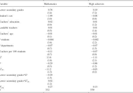
4.5. The Education Production Function Revisited (II)
The alternative interpretation of the estimation results from Eq. (15) is that rent seeking occurs for the speciali-zation subjects. In this case the estimated grading para-meter coefficients reported in Section 4.3 will be biased. The bias is due to correlation between the grading para-meter and the residual, generated by the unobserved student characteristics which determine the grading para-meter. To deal with this problem, instruments for the teacher grading parameter are generated from Eq. (15) and included in Eq. (14). Since the students’ initial aver-age level of knowledge is significantly associated with teachers’ grading, but not with student achievement, identification might be possible.
subjects are reported in Table 9. (We do not consider that endogeneity of the grading parameter is a problem for Norwegian language.)
As can be seen, the coefficients of the instruments are small and insignificant in all specifications. Formal F-tests suggest that one cannot reject the hypothesis that the coefficients of the instruments are equal to zero. We have generated alternative instruments by including interaction terms in Eq. (15), but in no case the instru-ments turn out to be significantly associated with student achievement. Formally, the tests imply that the grading parameters should be treated as exogenous, that is, the equation estimated in Section 4.3 seems to be the cor-rect equation.
Unfortunately, the evidence provided by these tests cannot be regarded as being very decisive. As can be seen from Table 9, the coefficients of the teacher charac-teristics become insignificant when the instruments are included in the estimated equation. This is an indication that the identification problems are not properly solved. The sample does not provide any additional variables that could help solve the identification problems.
Table 9
The education production function revisited (II)t-statistics in parentheses
Variable Mathematics High achievers
Lower secondary grades 0.78 0.19
(3.4) (7.2)
Student’s sex 21.99 20.08
(3.0) (0.8)
Teachers’ education 0.02 0.01
(0.9) (1.2)
Laudable teachers 0.01 0.01
(0.5) (1.4)
Teachers’ age 20.01 20.01
(0.1) (0.2)
# students 20.004 20.002
(3.6) (2.2)
# departments 20.07 20.07
(0.7) (1.5)
Teachers per 100 students 20.11 20.07
(0.7) (0.9)
G3 13.6 21.11
(1.6) (2.1)
gs 20.29 20.86
(0.3) (1.2)
G3
IV 211.2 20.03
(1.3) (0.2)
Lower secondary grades*G3 20.29
(1.5) Lower secondary grades*G3
IV 0.02
(1.2) R2
avg 0.27 0.13
N 332 559
5. Concluding Remarks
The understanding of the incentives facing students in existing school systems is probably a necessary con-dition for successful school reforms. In this paper we have focused on the teachers’ grading practices. Our point of departure is the Correa and Gruver’s model (1987) in which grades are conceptualized as a policy instrument for the teacher trying to manipulate a stud-ent’s studying time. Since students have strong incen-tives to press for easy grading, the basic model is aug-mented with rent seeking students. In this set up, teacher quality is decomposed into teaching quality and teacher strength. Teaching quality is linked to the achievement production function and teacher strength is defined as the teachers’ ability to withstand students’ pressure for easy grading.
laudability. The effects are rather large. It should be noted that teacher experience seems to matter only when teacher laudability is included in the estimated equation. We provide evidence that the teachers’ grading prac-tices are closely related to teacher characteristics. Two alternative explanations are offered; the first emphasizes that different types of teachers have different knowledge about the consequences of grading, while the second emphasizes that students press for easy grading and that the teachers’ ability to withstand pressure varies with teacher characteristics. The former explanation is con-sistent with the Correa and Gruver’s model where grad-ing is as a teacher’s policy variable. The latter expla-nation is consistent with the modified model where grading is endogenous. A formal statistical test indicates that the former explanation should be preferred.
What are the consequences of the teachers’ grading for student achievement? Treated as an exogenous variable, grading is shown to have a significant and substantial effect on student achievement. Hard grading improves student achievement, and the largest effect seems to be for high achieving students. The results complement our understanding of teacher characteristics: The estimation of the standard education production function has ident-ified teacher laudability and experience as important determinants of student achievement; the new evidence indicates that a direct effect of these characteristics goes through teaching quality and that an indirect effect goes through grading.
We have given several reasons why these results should not be regarded as definitive. The most pertinent question seems to be whether the revealed grading effect reflects a failure to control properly for teaching quality. Knowing that Montmarquette and Mahseredjian (1989) face this problem in their application of the Correa and Gruver’s model, we have deliberately chosen a sample with a very rich characterization of the teachers. Never-theless we cannot be sure that important dimensions of teaching quality have not been missed. The other main problem is whether the revealed grading effect reflects a failure to control for student rent seeking. Even though this possibility is formally rejected, we have given reasons why further investigations are required.
Thus, the results provided in this paper should not be used for policy purposes unless confirmed by further analyses. Further analyses should highlight the issues only touched upon here. The following argument illus-trates what we have in mind. Our findings emphasize the importance of information. It seems that only the laud-able and most experienced teachers know the true relationship between grading and real achievement. An optimistic view is that more information about effective grading practices will generate improvements in student achievement. There are two reasons why such an infor-mation-based reform could fail. First, the grading prac-tices may be embodied in teacher characteristics and
can-not be changed unless the teacher characteristics are changed. Second, the incentives faced by teachers and students, for instance the teachers’ costs of deviating from the best practices or the students’ gains from engag-ing in rent seekengag-ing, might be bindengag-ing constraints. Unless the importance of these types of factors has been clearified, the policy recommandations will not rest on firm ground.
Acknowledgements
The author is grateful to Jørn Rattsø and seminar parti-cipants in Trondheim for comments on earlier drafts of this paper. Comments by two anonymous referees were very useful in revising the paper. The author remains solely responsible for any errors in the text.
Appendix A
Data and variables
The data are provided by Nordland county, which is one of a total of 19 counties in Norway. 15 out of 16 schools providing academic subjects are included. The data describe the students who entered the upper second-ary schools in 1987 and finished in 1990. At the outset all students are included, but approximately 10 percent are left out due to missing observations. The students missing are drop-outs and students who have moved between schools during the period 1987–90.
The variable definitions are:
Exam results/Norwegian language: The average of the exam grades given to two essays, one in each of the two versions of the Norwegian language. All students are obliged to take both exams.
Teacher grading/Norwegian language: The average of the teacher’s grades for the two versions of the Norwegian language.
Exam results/specialization subjects: The average of the exam grades in the specialization subjects. All students are obliged to take an exam in at least one, often two, of his/her specialization subjects (mathematics, social studies, foreign language). Teacher grading/specialization subjects: The average of the teachers’ grades in the specialization subjects. The average includes only the student’s exam sub-jects.
Teachers’ education: The percentage of teachers hav-ing a master’s degree.
Laudable teachers: The percentage of teachers having laudable exam results on average from the university. Teachers’ age: The average age of the teachers in the teaching staff.
# students: The number of students in the academic department.
# departments: The number of departments within the combined school ( 5 the academic department
1a number of vocational departments. The number of vocational departments varies from 1 to 5 in this study.)
Teachers per 100 students: Teacher manyears to teaching exclusively divided by the number of stu-dents and multiplied by 100, i.e. all teacher input to other activities than teaching in the classroom are separated out.
Appendix B
Student response to teacher’s teaching time, the CES case
We basically follow Correa and Gruver’s presentation of the CES case, but include rent seeking as a stud-ent’s option.
Given the student CES utility function with elasticity of substitutionss51/(11b),
us5[q
1(ws)−b1q2(os)−b]−1/b, (B.1)
and CES achievement function with elasticitysv51/(1
1g),
v5[p1e−g1p2a−g]−1/g, (B.2)
and the grading function
ws5(12a)G(r)1aGT1gs(v23) (B.3)
and the time constraint
ks5e1r1os (B.4)
we will solve for the optimale*and r*.
Eq. B.(1) can be simplified by a monotonic transform-ation so that
ms5(us)−b/q
15(ws)−b1q(os)−b, whereq (B.5)
5q2/q1.
Minimizingmsis equivalent to maximizingus.
Substitut-ing Eq. B.(2), B.(3), B.(4) into Eq. B.(5) and takSubstitut-ing the first order conditions yields:
q5gsdv/de[(k2r2e)/(ws)]b 115f (B.6)
q5(12a)dG/dr[(k2r2e)/(ws)]b 115h (B.7)
The effect of teacher’s teaching time a9 on student’s studying time e*and rent seeking timer*can be found
by solving fordeanddr in the set of equations
fe9de1fr9dr1fa9da50 (B.8)
he9de1hr9dr1ha9da50 (B.9)
The partial derivatives are:
fe9 5g
s[(k2r2e)/(ws)]b[(b
11)(1/w)(dv/de)(212(k2r (B.10)
2e)(1/w)(dw/de))1d2v/de2((k2r2e)/w)]
fr9 5gs(b 11)(dv/de)(1/w)[(k2r
2e)/(ws)]b[212(k2r2e)(dG/dr)(1 (B.11)
2a)(1/ws)],0
fa9 5gs[(k2r2e)/(ws)]b 11[2(b (B.12)
11)(1/w)(dv/de)(dw/da)1d2v/dade]
he9 5(12a)(b 11)(dG/dr)(1/w)[(k2r
2e)/(ws)]b[212(k2r2e)(dw/de)(1/w)] (B.13)
,0
hr9 5(12a)[(k2r2e)/(ws)]b[2(b
11)(dG/dr)(1/w)(11(k2r (B.14)
2e)(dw/dr)(1/w))1(k2r
2e)/(ws)(d2G/dr2)],0
ha9 5 2(12a)(b 11)(1/w)[(k2r (B.15)
2e)/(ws)]b 11(dG/dr)(dw/da),0
It is clear thatfe9,fr9,he9,hr9and ha9are negative. The
sign of fa9depends on the sign of the second factor of
Eq. B.(12). As in Correa and Gruver it follows that
fa9> 0iffss>sv (B.16)
That is,fa9is positive if and only if the elasticity of
sub-stitution in the student’s utility function is larger than the elasticity of substitution in the achievement function.
From the Eq. B.(8), B.(9) we have that
de5da(ha9fr9 2hr9fa9)/(hr9fe9 2he9fr9) (B.17)
dr5da(he9fa9 2ha9fe9)/(hr9fe9 2he9fr9) (B.18)
It follows that increased teaching time a9 yields increased studying time if fa9 > 0 and hr9fe9 > he9fr9.
Under the same conditions, increased teaching time yields decreased rent seeking time.
Now,fa9> 0 if achievement and leisure are close
seek-ing time and studyseek-ing time on the equilibrium conditions Eq. B.(6), B.(7) are larger than the indirect cross effects. Thus, the essential points seem to be that the students’ response to increased teaching time may vary across stu-dents, and also across teachers if the teachers apply dif-ferent teaching technologies.
The effects of improved teaching quality (a positive shift in the achievement production function) is anal-ogous to increased teaching time. Now we investigate the effects of increased teacher strength, which is rep-resented by the shift parameteruin the functionG(r,u). The effects of increased teacher strength on student’s studying timee*and rent seeking timer*can be found
by solving fordeanddr in the set of equations
fe9de1fr9dr1fu9du 50 (B.19)
he9de1hr9dr1hu9du 50 (B.20)
The solutions are
de5du(hu9fr9 2hr9fu9)/(fe9hr9 2he9fr9) (B.21)
dr5du(he9fu9 2hu9fe9)/(fe9hr9 2he9fr9) (B.22)
where
fu9 5 2gs(b 11)(dv/de)(1/w)[(k2r (B.23)
2e)/ws]b 11(dw/du),0
hu9 5(12a)[(k2r
2e)/ws]b 11[d2G/(drdu)2(b (B.24)
11)(dG/dr)(dw/du)(1/w)]
and the other partial derivatives are given above.Assum-ing that the denominators in Eq. B.(21), B.(22) are posi-tive, the student’s response to increased teacher strength (du,0) depends on the sign ofhu9. Ifhu9> 0, thende> 0 anddr ,0. Now,
hu9> 0iff1/(1 (B.25)
1b) > (dG/dr)(dw/du)(1/w)/(d2G/drdu)
That is, if achievement and leisure time are close substi-tutes in the student’s utility function, and the rent seeking response to increased teacher strength is rather small, the student will increase the studying time and reduce the rent seeking time.
References
Bishop, J. H. (1989) Why the apathy in American high schools? Educational ResearcherJan–Feb., 6–10.
Bonesrønning, H., 1996. Combined school characteristics and student achievement: Evidence from Norway. Education Economics 4 (2), 143–160.
Brown, B. and Saks, D. (1980) Production technologies and resource allocation within classrooms and schools: Theory and Measurement. In The Analysis of Educational Pro-ductivity(Edited by Dreeben, R. and Thomas, J. A.). Cam-bridge, Mass: Ballinger.
Correa, H., Gruver, G.W., 1987. Teacher-student interaction: a game theoretic extention of the economic theory of edu-cation. Mathematical Social Science 13, 19–47.
Ehrenberg, R.G., Brewer, D.J., 1995. Did teachers’ verbal ability and race matter in the 1960s? Coleman revisited. Economics of Education Review 14 (1), 1–21.
Farkas, G., Hotchkiss, L., 1989. Incentives and disincentives to subject matter difficulty and student effort: course grade determinants across the stratification system. Economics of Education Review 8 (2), 121–132.
Hanushek, E. (1986) The economics of schooling: production and efficiencies in public schools. Journal of Economic Literature,XXIV, 1141–1177.
Hanushek, E. and Taylor, L. (1990) Alternative assessments to the performance of schools.Journal of Human Resources,
XXV(2), 179-201.
Heckman, J., 1979. Sample selection bias as a specification error. Econometrica 47, 153–161.
Hoenack, S.A., 1994. Economics, organizations and learning: research directions for the economics of education. Econom-ics of Education Review 13 (2), 147–162.