DETERMINING PLANE-SWEEP SAMPLING POINTS IN IMAGE SPACE
USING THE CROSS-RATIO FOR IMAGE-BASED DEPTH ESTIMATION
B. Rufa,b, B. Erdnuessa,b, M. Weinmannb
aFraunhofer IOSB, Video Exploitation Systems, 76131 Karlsruhe, Germany -(boitumelo.ruf, bastian.erdnuess)@iosb.fraunhofer.de
bInstitute of Photogrammetry and Remote Sensing, Karlsruhe Institute of Technology, 76131 Karlsruhe, Germany - (boitumelo.ruf, bastian.erdnuess, martin.weinmann)@kit.edu
Commission II, WG II/4
KEY WORDS:depth estimation, image sequence, plane-sweep, cross-ratio, online processing
ABSTRACT:
With the emergence of small consumer Unmanned Aerial Vehicles (UAVs), the importance and interest of image-based depth estimation and model generation from aerial images has greatly increased in the photogrammetric society. In our work, we focus on algorithms that allow an online image-based dense depth estimation from video sequences, which enables the direct and live structural analysis of the depicted scene. Therefore, we use a multi-view plane-sweep algorithm with a semi-global matching (SGM) optimization which is parallelized for general purpose computation on a GPU (GPGPU), reaching sufficient performance to keep up with the key-frames of input sequences. One important aspect to reach good performance is the way to sample the scene space, creating plane hypotheses. A small step size between consecutive planes, which is needed to reconstruct details in the near vicinity of the camera may lead to ambiguities in distant regions, due to the perspective projection of the camera. Furthermore, an equidistant sampling with a small step size produces a large number of plane hypotheses, leading to high computational effort. To overcome these problems, we present a novel methodology to directly determine the sampling points of plane-sweep algorithms in image space. The use of the perspective invariant cross-ratio allows us to derive the location of the sampling planes directly from the image data. With this, we efficiently sample the scene space, achieving higher sampling density in areas which are close to the camera and a lower density in distant regions. We evaluate our approach on a synthetic benchmark dataset for quantitative evaluation and on a real-image dataset consisting of aerial imagery. The experiments reveal that an inverse sampling achieves equal and better results than a linear sampling, with less sampling points and thus less runtime. Our algorithm allows an online computation of depth maps for subsequences of five frames, provided that the relative poses between all frames are given.
1. INTRODUCTION
In recent years, the importance and interest of image-based depth estimation and model generation from aerial images has greatly increased in the photogrammetric so-ciety. This trend is especially due to the emergence of small consumer Unmanned Aerial Vehicles (UAVs), which easily and cost-effectively allow the capturing of images from an aerial viewpoint. These images are used to gen-erate three-dimensional models depicting our surrounding and, in turn, using such models alleviates various appli-cations such as urban reconstruction (Blaha et al., 2016; Musialski et al., 2013; Rothermel et al., 2014), urban nav-igation (Serna and Marcotegui, 2013), scene interpreta-tion (Weinmann, 2016), security surveillance (Pollok and Monari, 2016) and change detection (Taneja et al., 2013). An important step in the process of model generation from imagery is the image-based depth estimation, commonly known as Structure-from-Motion (SfM). While the accu-racy achieved by state-of-the-art SfM algorithms is quite impressive, such results come at the cost of performance and runtime, in particular when it comes to high resolution dense depth estimation.
In our work, we focus on algorithms that allow an on-line image-based dense depth estimation from video
se-quences. Online processing does not necessarily aim to estimate depth maps for each input frame of the video sequence, but rather for every key-frame which are typi-cally generated at 1Hz - 2Hz. This enables the direct and live structural analysis of the depicted scene. As video sequences allow the use of multiple images for reconstruc-tion, we employ a plane-sweep algorithm for image match-ing. Apart from its ability of true multi-image matching (Collins, 1995), the plane-sweep algorithm can efficiently be optimized for general purpose computation on a GPU (GPGPU), necessary in order to achieve sufficient per-formance for online processing. Furthermore, urban sur-roundings are well-suited for an approximation by planar structures. The accuracy achieved and the runtime needed by SfM algorithms mainly depend on two factors: One is the optimization step employed after the image matching, which determines the per-pixel depth value of the result-ing depth map. The second factor is the samplresult-ing of the scene space.
sam-pled efficiently, especially when it comes to oblique aerial images due to the large scene depth. Moreover, a typi-cal characteristic of perspective cameras is that sizes and lengths of objects become smaller as these objects move away from the camera. And as the input data are the im-ages, it is vital that the sampling points are selected in image space, instead of in scene space.
In this paper, we present a methodology to derive the sam-pling points of plane-sweep algorithms directly from points in image space. Our contributions are:
• The use of the perspective invariant cross-ratio to de-rive the sampling points of plane-sweep algorithms from correspondences in image space.
• The employment of a true multi-image plane-sweep algorithm for the image-based depth estimation of ur-ban environments from aerial imagery.
This paper is structured as follows: In Section 2, we briefly summarize related work. Thereby, we give a short overview of different sampling strategies in image-based depth estimation, and we also explain how the plane-sweep algorithm differs from tensor-based strategies. Further-more, we introduce different work that has been done in re-construction of urban environments, especially from aerial imagery. In Section 3, we give a detailed description of our methodology. We present our experimental results in Section 4 and provide a discussion in Section 5. Finally, we give a short summary and an outlook on future work in Section 6.
2. RELATED WORK
In this section, we first provide a short introduction into different methodologies for image-based depth estimation. We explain how the plane-sweep algorithm differs from the conventional exploitation of epipolar geometry and why it is considered as a true multi-image matching algorithm. In the second part of this section, we will give a brief overview on previous work done in image-based reconstruction of urban environments both from ground-based and aerial imagery.
2.1 Image-Based Depth Estimation
A common approach for dense stereo reconstruction is to exploit the epipolar geometry between two images. The intrinsic calibration of the camera and the relative ori-entation between both images allow to reduce the search space for pixel correspondences to a one-dimensional path, called the epipolar line. The so-called fundamental matrix determines this epiploar line in the matching image, cor-responding to a given pixel in the reference image. In the past years, numerous algorithms with different optimiza-tion strategies have been developed to compute optimal disparity and depth maps from a two-view stereo setup. Scharstein and Szeliski (2002) introduce a taxonomy that groups these algorithms according to their strategies.
One drawback of using only two views is that a left-right consistency check is required in order to find occlusions,
which inevitably increases the computational effort. To overcome this problem, Kang et al. (2001) stated that by using multiple views the consistency check can be omit-ted, if a left and right subset with respect to the reference image is independently used for image matching. If the reference frame, for which the depth is to be computed, is located in the middle, it can be assumed that if an object is occluded in the matching image on the one side of the reference frame, it is most likely visible in the image on the other side. This is particularly applicable when recon-structing 2.5D data, such as buildings and elevation, with no overhanging objects.
The trifocal and quadrifocal tensors allow to extend the epipolar geometry to three and four views respectively. While the trifocal tensor can still be computed efficiently, the quadrifocal tensor is rather unpractical (Hartley and Zisserman, 2004). Furthermore, tensor-based methods are restricted to a maximum of four views. To achieve a true multi-image matching, Collins (1995) introduced the so-called plane-sweep algorithm, in which a plane is swept through space. For each position of the plane, the match-ing images are perspectively warped into the reference frame via the plane-induced homography. The idea is that if the plane is close to an object in scene space, the warped matching images and the reference image will align in the corresponding areas. The optimal plane position for each pixel can efficiently be found by minimizing the matching costs. The final per-pixel depth is then computed by inter-secting the ray through the pixel with the optimal plane. This algorithm is suitable for different sweeping directions, i.e. plane orientations, which can be aligned with the ori-entation of objects which are to be reconstructed. The approach of sampling the scene with different planes is of-ten used in the image-based depth estimation, especially when it comes to multi-image matching (Baillard and Zis-serman, 2000; Pollefeys et al., 2008; Ruf and Schuchert, 2016; Sinha et al., 2014; Werner and Zisserman, 2002).
2.2 Urban Reconstruction
In recent years, much effort has been spent on the field of urban reconstruction. We group the previous work into two categories based on their input data. On the one hand we consider work that is based on ground-based imagery, and on the other hand we look at work which uses aerial imagery for urban reconstruction. In their work, Werner and Zisserman (2002) use a plane-sweep approach to re-construct buildings from a ground-based viewpoint. A line detection algorithm is used to determine plane orientations by finding vanishing points. Given the orientations, the planes are swept to estimate fine structures.
Pollefeys et al. (2008) as well as Gallup et al. (2007) intro-duce a plane-sweep approach with multiple sweeping direc-tions to reconstruct urban fa¸cades from vehicle-mounted cameras. They utilize an inertia system and vanishing points found in the input images to estimate the orien-tation of the ground plane as well as the orienorien-tation of the fa¸cade planes. While Pollefeys et al. (2008) find the opti-mal planes by determining a Winner-Takes-It-All (WTA) solution, Gallup et al. (2007) employ the optimization of an energy functional to obtain the optimal planes.
piecewise planar reconstruction under the assumption that the building fa¸cades are standing perpendicular to each other. Furthermore, the piecewise planar reconstruction of urban scenery from ground-based imagery is done by Sinha et al. (2009) and Gallup et al. (2010). They fit local planes into sparse point clouds or initial depth maps and determine the depth map by employing a final multi-label MRF optimization.
Baillard and Zisserman (2000) apply a plane-fitting strat-egy for a 3D reconstruction of buildings from aerial images with a quasi-nadir view point. They extract the edges of buildings by line detection and try to fit so-called half-planes through these edges. In order to estimate the pitch angle of these half-planes, they apply a similarity matching between multiple views warped by homographies induced by the planes. In a final step, they fuse adjacent half-planes to compute the building models.
The use of Digital Elevation Models (DEMs) to reconstruct urban buildings from aerial imagery is addressed by Zebe-din et al. (2008). Their approach does not utilize image matching but rather tries to extract the buildings from the DEMs. They use line segments, which are determined from the aerial imagery, to approximate the buildings with geometric primitives.
In their work, Haala et al. (2015) describe an extraction of 3D urban models from oblique aerial images. They in-troduce a modification of the semi-global matching (SGM) algorithm (Hirschmueller, 2008) that enables a coarse-to-fine optimization, in order to overcome the problem of high computational complexity due to occurring occlusions and large viewpoint changes, inherent to oblique imagery.
Hofer et al. (2017) introduce an efficient abstraction of 3D modelling by using line segments. Their methodology performs well in urban environments as buildings and man-made objects are very suitable to be abstracted by line segments.
PMVS (Furukawa and Ponce, 2010) and SURE (Rother-mel et al., 2012) are examples of software tools for state-of-the-art dense multi-view stereo (MVS) reconstruction. PMVS reconstructs the scene with a large number of small patches. Similar to plane-sweep depth estimation, it opti-mizes the orientation and location of the patches by per-forming multi-image matching. SURE, on the other hand, performs a triangulation of pixel correspondences in multi-ple views in order to reconstruct the depicted scene. These software tools are typically designed for offline processing, meaning that for the reconstruction all input images are considered to be available. Furthermore, while offline re-constructions commonly produce results with higher accu-racy, their computation takes several minutes to hours, de-pending on the size and complexity of the captured scene. As we aim to perform an online depth estimation, i.e. while the image sequence is captured, we can only assume to have fewer input images and are restricted in the com-plexity of optimization in order to keep up with the input sequence.
3. METHODOLOGY
Our plane-sweep algorithm for image-based depth estima-tion is based on the one described by Ruf and Schuchert
(2016). Given a set of five input images with correspond-ing projection matrices Pi= K [Riti], we compute a depth map for an identified reference frame which is typically the middle frame of a short image sequence. As we are using video imagery, the intrinsic camera matrix K is the same for all images. The algorithm sweeps a plane through the 3D Euclidean scene spaceE3and warps each matching im-age by the plane-induced homography H into the reference frame:
H = K·R−tn
T
d ·K
−1
(1)
where R,t = relative rotation and translation n = plane normal vector
d= plane distance from the reference camera
This builds up a three-dimensional matching cost volume of size W ×H× |Γ|, whereW and H correspond to the image width and height, respectively. The set of planes, which are used for reconstruction, is denoted by Γ⊂E3. Thus, |Γ|denotes to the number of planes. We optimize the cost volume with an eight path semi-global match-ing (SGM) aggregation, as introduced by Hirschmueller (2008), in order to determine the per-pixel optimal plane and with it the depth. As similarity measures, we use the sampling insensitive matching cost proposed by Birch-field and Tomasi (1999). This is a sub-pixel accurate absolute-difference cost function, which is cheep to com-pute and yet provides good results for SGM-based methods (Hirschmueller and Scharstein, 2007).
As stated by Equation 1 the plane-sweep algorithm is con-figured by two parameters. One is given by n which de-notes the orientation and thus the sweeping direction of the planes. This parameter can be used to adjust the al-gorithm to known scene structures. While the presented methodology can be applied to any sweeping direction, we use a frontoparallel plane orientation for the sake of brevity and simplicity. The second parameterdrepresents the distances of each plane from the optical centre of the reference camera, i.e. the step sizes with which the planes are swept through scene space along the normal vector.
p1 p2 p3 p4
l0
l1
l2
Δ(p1, p2)
δ(k, l) C
a b c d
A straight-forward parametrization would be to select the parameter in scene space according to the structure and the resolution with which the scene is to be sampled. While a small step size might suggest a thorough sam-pling of the scene, it does not guarantee a higher accuracy. Depending on the baseline between the cameras, multiple sampling points might be projected onto the same pixel, resulting in ambiguities between multiple plane hypothe-ses. Furthermore, due to the perspective projection of the cameras, it is necessary to decrease the sampling step as the plane comes closer to the camera.
In order to reduce these ambiguities and sample the scene according to the input data, it is a common approach in state-of-the-art literature to sample the scene with an in-verse depth. Yang and Pollefeys (2003) formulate the cal-culation of inverse depth given the disparity for a stereo setup with frontoparallel cameras. Even though their for-mulation incorporates different camera setups, it is not applicable for non-frontoparallel planes as the plane ori-entation is not considered when computing the distances of the planes with respect to the reference camera. While Gallup et al. (2007) and Pollefeys et al. (2008) consider different plane orientations, they determine the distance of consecutive planes by comparing the disparity change caused by the image warpings of the respective planes. In order to reduce the complexity they only consider the im-age borders, as they induce the largest disparity change. Nonetheless, it requires a preliminary warping in order to find the set of planes with which the scene is sampled.
In contrast, we aim to derive the locations of the sam-pling planes directly from correspondences in image space
I ∈ R2. Given an homogeneous image point ˜x ∈ Irefin the reference frame and multiple homogeneous sampling points ˜x′
i ∈ Ikin one of the other camera frames, we aim to find the plane distancesdi, with respect to the reference camera, of the corresponding plane-induced homographies Hi, so that ˜x= Hi·x˜′iholds. An intuitive approach to find the corresponding planes would be to triangulate between ˜
xand ˜x′
i. Yet, the effort of triangulation can be avoided by using the cross-ratio within the epipolar geometry to determine the distance parametrization of the planes.
3.1 Cross-Ratio as Invariant Under Perspective Projection
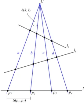
The cross-ratio describes the ratio of distances between four collinear points. While the distances between these points change under the perspective projection, their rela-tionship relative to each other, i.e. the cross-ratio, is invari-ant. Given are four pointsp1,p2,p3 andp4 on a straight line l0 as depicted in Figure 1, which are perspectively projected onto further non-parallel lines, such asl1andl2. With the known oriented distances ∆(pi, pj) between two points pi and pj, the cross-ratio is determined according to:
CR(p1, p2, p3, p4) =
∆(p1, p3)∆(p2, p4) ∆(p1, p4)∆(p2, p3)
(2)
This ratio is the same on all three lines. Furthermore, with the pairwise enclosed anglesδ(k, l) between the raysa,b,
R, t
C2
C1
Iref Πmin Πmax
lx Πi
cΠ
x Xmin
Xi
Xmax
e1 x'min x'i
x'max
Vx
Ve1 Vx'min Vx'i
Vx'max
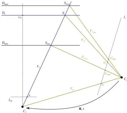
Figure 2. The use of the cross-ratio to determine the dis-tance parameter of the sampling planes.
candd, going through the centre of projectionCand the four points, the cross-ratio can be extended to:
CR(p1, p2, p3, p4) =CR(a, b, c, d)
= sin(δ(a, c)) sin(δ(b, d)) sin(δ(a, d)) sin(δ(b, c))
(3)
3.2 Determining Plane Distances with Cross-Ratio
To determine the plane distances relative to the optical centre of the reference camera with use of the cross-ratio, we assume that two camerasC1 andC2 with known pro-jection matrices are given, as depicted in Figure 2. We select C1 to be the reference camera, centering the coor-dinate system in its optical centre, so that P1 = K [I 0]. In case of a multi-camera setup, we choose C2 to be the camera inferring the largest image offset compared to the reference frame. This is typically one of the most distant cameras.
Furthermore, two planes Πminand Πmax are known which limit the Euclidean sweep space. With a given image point x in the reference frame we can compute the ray
Vx through the camera centre and the image point. In-tersectingVx with the planes Πmin and Πmax gives us the corresponding scene points Xmin and Xmax. Projecting the optical centre ofC1 as well as the scene pointsXmin andXmax onto the image plane ofC2gives us the epipole
e1 and the two image points x′min andx′max which all lie on the epipolar linelxcorresponding tox.
Our aim is to find the distancesdimeasured fromC1of all planes Πi between Πmax and Πmin, so that lx is sampled linearly withx′
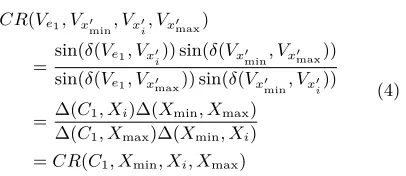
we apply Equations 2 and 3:
CR(Ve1, Vx′
min, Vx′i, Vx′max)
= sin(δ(Ve1, Vx′i)) sin(δ(Vx′min, Vx′max))
sin(δ(Ve1, Vx′max)) sin(δ(Vx′min, Vx′i))
= ∆(C1, Xi)∆(Xmin, Xmax) ∆(C1, Xmax)∆(Xmin, Xi) =CR(C1, Xmin, Xi, Xmax)
(4)
Resolving Equation 4 gives usXi∈Vx. Furthermore, due to CR(C1, Xmin, Xi, Xmax) =CR(C1, dmin, di, dmax), and as the plane distance is given relative toC1, we can derive
di according to:
di·(dmax−dmin)
dmax·(di−dmin)
=sin(δ(Ve1, Vx′i)) sin(δ(Vx′min, Vx′max))
sin(δ(Ve1, Vx′max)) sin(δ(Vx′
min, Vx′i))
.
(5)
As already stated, the presented approach is not re-stricted to a frontoparallel plane orientation, but can be applied to all kinds of orientations. It is important to use
CR(Ve1, Vx′
min, Vx′i, Vx′max) in Equation 4 to account for all
possible setups betweenC1andC2, ase1would flip to the side ofx′
maxifC1is behindC2. Furthermore, to guarantee a maximum disparity change between succeeding planes for all pixels inIref,xshould be chosen as the pixel which generates the largest disparity when warped from C1 to
C2. This is typically one of the four corner pixels ofIref.
4. EXPERIMENTS
To evaluate the performance of our methodology, we use two different test datasets. First, we consider the New Tsukuba Stereo Benchmark (NTSB)(Martull et al., 2012), which provides a video of a camera flight through a thetic indoor scene. Due to the fact that this is a syn-thetic test dataset, it provides a reference in the form of camera poses and high-quality groundtruth depth maps for each input frame. These are used for quantitative eval-uation. To test our methodology on real scenario data, we use aerial images of a transporter and container on our premises, captured by a DJI Phantom 3.
In order to reduce image noise, the input images are down-sampled by a factor of 0.8, which is determined empiri-cally. Our algorithm runs on grayscale images. The image matching, as well as the SGM optimization are parallelized for general purpose computation on a GPU (GPGPU) with OpenCL. All experiments are performed on a desktop com-puter with an Intel Core i7-5820K CPU @ 3.30GHz and a Nvidia GTX980 GPU. Please note that for a better map-ping of our algorithm onto the architecture of the GPGPU the number of sampling planes is always rounded up to the nearest multiple of the warp size, which in case of the used GPU is 32.
We evaluate the performance of our proposed methodology for determining the sampling points of the plane-sweep al-gorithm in image space against results obtained by a linear
sampling in scene space. For quantitative assessments of the depth-error against the groundtruth of the NTSB, we employ an averaged relative L1 accuracy measure:
L1-rel(z,ˆz) = 1
W× H
X
i
|zi−zˆi| ˆ
zi
(6)
where z = depth estimate ˆ
z = groundtruth
W, H = image size
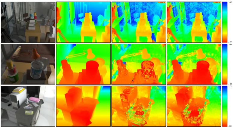
The original image size of the images used within the NTSB is 640×480 pixels. Figure 3 depicts a qualita-tive comparison between a linear sampling in scene space with a plane step size of 2 units and a linear sampling in image space according to the proposed methodology with a disparity change of maximum 1 pixel. We test our methodology on three subsequences of five frames around the Frames 295, 380 and 845 of the NTSB. These sub-sequences provide similar views on the scene as can be expected when performing image-based depth estimation on aerial imagery with an oblique viewpoint. In addition to the estimated depth maps, Figure 3 holds the refer-ence frame as well as the corresponding groundtruth depth map. The depth maps are color coded in the HSV color space, going from red to blue. The penalization weights in the SGM algorithm are set toP1 = 0.05 andP2 = 0.1 for the NTSB. These weights have empirically been tested to provide the best results for this dataset.
Table 1 holds a quantitative comparison between four dif-ferent sampling configurations of the image-based depth estimation performed on the NTSB. Besides the configura-tions (a) and (d) which correspond to the results depicted in Figure 3, configuration (b) lists the results of a linear sampling in scene space with the same number of planes as used in (d). Furthermore, we list the results of config-uration (c) in which the linear sampling in image space is reduced to a maximum disparity change of 2 pixels.
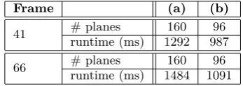
In terms of our evaluation on aerial imagery, we provide a qualitative evaluation in Figure 4. We test on two refer-ence frames depicting the same scene, but captured from different heights. For reference Frame 41 we use a linear sampling in image space of 0.04 units, while for Frame 66 we use a step size of 0.02 units. The original frame size we use is 960×720 pixels. The weights of the SGM opti-mization are empirically set toP1 = 10 andP2 = 20. To account for changes in exposure, we perform a histogram equalization on the input images. A quantitative compar-ison listing the number of planes used and the runtime is given in Table 2.
5. DISCUSSION
402
85 464
44
104 521
Figure 3. Qualitative evaluation on three sequences of the New Tsukuba Stereo Benchmark (NTSB). Row 1: Frame 295. Row 2: Frame 380. Row 3: Frame 845. Column 1: Reference frame. Column 2: Groundtruth depth map. Column 3: Estimated depth map with linear sampling of 2 units in scene space. Column 4: Estimated depth map with linear sampling of<1 pixel along the epipolar line in image space.
Table 1. Quantitative evaluation between four different configurations on the NTSB.(a)Linear sampling in scene space, with a step size of 2 units. (b)Linear sampling in scene space with 96 planes. (c)Linear sampling in image space with a disparity change of max. 2 pixels. (d)Linear sampling in image space with a disparity change of max. 1 pixel.
Frame (a) (b) (c) (d)
295
L1-rel 0.094 0.094 0.096 0.095
# planes 160 96 64 96
runtime (ms) 277 152 92 145
380
L1-rel 0.223 0.153 0.130 0.126
# planes 224 96 64 96
runtime (ms) 452 142 93 142
845
L1-rel 0.169 0.129 0.109 0.109
# planes 224 96 64 96
runtime (ms) 465 138 95 142
depth. Employing a linear sampling in scene space could lead to ambiguities in distant regions as multiple sampling points would project onto the same pixel if the step size is too small. The objective of our methodology is to use the available data, i.e. the images, to directly determine the sampling points of the plane-sweep algorithm. Thus, reducing the runtime without a loss in accuracy by elimi-nating unnecessary sampling points.
Figure 3 depicts a comparison between the results obtained by a linear sampling in scene space with a step size of 2 units (Column 3) and a linear sampling in image space with a maximum disparity change of 1 pixel (Column 4), which is equivalent to an inverse sampling in scene space. While the results for the subsequence around Frame 295 (Row 1) do not reveal a considerable change in the qual-ity between both sampling methods, a comparison of the results for the other subsequences shows a great difference in the depth maps. Especially in close regions our
pro-posed method achieves depth maps with higher quality. This is due to the inverse sampling of the scene, leading to smaller step sizes between consecutive planes when ap-proaching the camera. The graph in Figure 5 depicts the sampling points which are obtained by a linear and in-verse sampling in scene space with the same number of planes. It clearly shows that inverse sampling achieved by the presented methodology uses less planes in distant re-gions, while increasing the sampling density with decreas-ing scene depth. Furthermore, as evaluated by Gallup et al. (2008), it is important to sample more thoroughly in areas of high-frequency textures, as can be seen when con-sidering the table cloth in Row 3 of Figure 3.
Table 1 confirms the results depicted in Figure 3. For Frame 295, the accuracy does not notably change between configurations (a) and (d) when using less planes. This can be attributed to the small number of objects that are in near vicinity of the camera. Yet, the runtime is clearly reduced, which is important when considering online ap-plications. In case of the subsequences around Frame 380 and Frame 845, an inverse sampling achieves considerably better results, while using less planes. This can also be ob-served by a comparison in Figure 3. The results for con-figuration (b) show that linear sampling with a reduced number of planes achieves slightly better results than con-figuration (a) due to less ambiguities, yet still doesn’t per-form better than inverse sampling. An increase in the maximum disparity change between consecutive planes, as tested in configuration (c), slightly reduces the accuracy, but nonetheless still achieves better results than a linear sampling.
an-4.2 7.2 3.5 9.5
Figure 4. Qualitative evaluation on aerial imagery between. Row 1: Frame 41. Row 2: Frame 66. Column 1: Reference frame. Column 2: Estimated depth map with linear sampling in scene space. Column 3: Estimated depth map with linear sampling along the epipolar line in image space.
Figure 5. Comparison between linear and inverse sampling in scene space.
gles. While the algorithm achieves adequate results on the first configuration with a slight oblique view (Row 1), a greater off-nadir angle (Row 2) leads to higher noise, due to the visible background. Furthermore, as we sample with a frontoparallel plane orientation, the ground in front of the container also leads to false estimations as the grass could not be matched properly due to the great difference in ori-entation between the planes and the ground. In a qualita-tive comparison between the different sampling methods, the inverse sampling proposed by our approach achieves results with slightly less variations and noise. This can be observed on the roof of the van in Row 1, as well as above the container in Row 2. Especially with respect to the reduction in runtime, as listed in Table 2, inverse sampling has shown to produce considerably better results than simple linear sampling.
6. CONCLUSION & FUTURE WORK
In this paper, we introduced a methodology to determine sampling points for image-based plane-sweep depth esti-mation directly in image space. Plane-sweep algorithms are typically parametrized by the direction and the step size at which the plane is swept through scene space. We utilize the cross-ratio, which is invariant under the
per-Table 2. Quantitative evaluation between four different configurations on aerial imagery. (a) Linear sampling in scene space with 160 planes. (b)Linear sampling in image space with a disparity change of max. 1 pixel.
Frame (a) (b)
41 # planes 160 96
runtime (ms) 1292 987
66 # planes 160 96
runtime (ms) 1484 1091
spective projection of cameras, to derive the position of the planes relative to the reference camera directly from points in image space. This allows us to sample the scene space between two delimiting plane configurations, given a maximum disparity displacement invoked by two con-secutive planes along the epipolar line. Our methodology generates an inverse sampling of the scene space, achiev-ing higher samplachiev-ing density in areas which are close to the camera and a lower density in distant regions. This guar-antees a more thorough sampling in areas which allow a more detailed reconstruction, while reducing unnecessary sampling points in areas where less disparity is induced. Such an inverse sampling is particularly important when considering scenes with large scene depth such as those de-picted in oblique aerial imagery. The experiments reveal that an inverse sampling achieves equal and better results than a linear sampling with less sampling points and thus less runtime.
References
Baillard, C. and Zisserman, A., 2000. A plane-sweep strategy for the 3d reconstruction of buildings from multiple images. In: International Archives of Photogrammetry and Remote Sensing, Amsterdam, The Netherlands, Vol. XXXIII-B2, IS-PRS, pp. 56–62.
Birchfield, S. and Tomasi, C., 1999. Depth discontinuities by pixel-to-pixel stereo.International Journal of Computer Vi-sion (IJCV)35(3), pp. 269–293.
Blaha, M., Vogel, C., Richard, A., Wegner, J. D., Pock, T. and Schindler, K., 2016. Large-scale semantic 3d reconstruction: an adaptive multi-resolution model for multi-class volumetric labeling. In: Proceedings of the IEEE Conference on Com-puter Vision and Pattern Recognition (CVPR), Las Vegas, NV, USA, IEEE, pp. 3176–3184.
Collins, R. T., 1995. A space-sweep approach to true multi-image matching. Technical report, University of Mas-sachusetts, Amherst, MA, USA.
Furukawa, Y. and Ponce, J., 2010. Accurate, dense, and robust multiview stereopsis. IEEE Transactions on Pattern Analy-sis and Machine Intelligence (TPAMI)32(8), pp. 1362–1376.
Furukawa, Y., Curless, B., Seitz, S. M. and Szeliski, R., 2009. Manhattan-world stereo. In: Proceedings of the IEEE Conference on Computer Vision and Pattern Recognition (CVPR), Miami, FL, USA, IEEE, pp. 1422–1429.
Gallup, D., Frahm, J.-M. and Pollefeys, M., 2010. Piecewise planar and non-planar stereo for urban scene reconstruction. In:Proceedings of the IEEE Conference on Computer Vision and Pattern Recognition (CVPR), San Francisco, CA, USA, IEEE, pp. 1418–1425.
Gallup, D., Frahm, J. M., Mordohai, P. and Pollefeys, M., 2008. Variable baseline/resolution stereo. In: Proceedings of the IEEE Computer Society Conference on Computer Vision and Pattern Recognition (CVPR), Anchorage, AK, USA, IEEE, pp. 1–8.
Gallup, D., Frahm, J.-M., Mordohai, P., Yang, Q. and Polle-feys, M., 2007. Real-time plane-sweeping stereo with multiple sweeping directions. In:Proceedings of the IEEE Conference on Computer Vision and Pattern Recognition (CVPR), Min-neapolis, MN, USA, IEEE, pp. 1–8.
Haala, N., Rothermel, M. and Cavegn, S., 2015. Extracting 3d urban models from oblique aerial images. In: Proceedings of the IEEE Joint Urban Remote Sensing Event (JURSE), Lausanne, Switzerland, IEEE, pp. 1–4.
Hartley, R. and Zisserman, A., 2004.Multiple view geometry in computer vision. Cambridge University Press.
Hirschmueller, H., 2008. Stereo processing by semiglobal match-ing and mutual information.IEEE Transactions on Pattern Analysis and Machine Intelligence (TPAMI)30(2), pp. 328– 341.
Hirschmueller, H. and Scharstein, D., 2007. Evaluation of cost functions for stereo matching. In: Proceedings of the IEEE Conference on Computer Vision and Pattern Recognition (CVPR), Minneapolis, MN, USA, IEEE, pp. 1–8.
Hofer, M., Maurer, M. and Bischof, H., 2017. Efficient 3d scene abstraction using line segments.Computer Vision and Image Understanding (CVIU)157, pp. 167–178.
Kang, S. B., Szeliski, R. and Chai, J., 2001. Handling occlu-sions in dense multi-view stereo. In:Proceedings of the IEEE Computer Society Conference on Computer Vision and Pat-tern Recognition (CVPR), Kauai, HI, USA, Vol. 1, IEEE, pp. 103–110.
Martull, S., Peris, M. and Fukui, K., 2012. Realistic CG stereo image dataset with ground truth disparity maps. In: Proceed-ings of the International Conference on Pattern Recognition (ICPR), Tsukuba, Japan, Vol. 111, pp. 117–118.
Musialski, P., Wonka, P., Aliaga, D. G., Wimmer, M., van Gool, L. and Purgathofer, W., 2013. A survey of urban reconstruc-tion. Computer Graphics Forum32(6), pp. 146–177.
Pollefeys, M., Nist´er, D., Frahm, J.-M., Akbarzadeh, A., Mor-dohai, P., Clipp, B., Engels, C., Gallup, D., Kim, S.-J., Mer-rell, P., Salmi, C., Sinha, S., Talton, B., Wang, L., Yang, Q., Stew´enius, H., Yang, R., Welch, G. and Towles, H., 2008. De-tailed real-time urban 3d reconstruction from video. Interna-tional Journal of Computer Vision (IJCV)78(2-3), pp. 143– 167.
Pollok, T. and Monari, E., 2016. A visual SLAM-based ap-proach for calibration of distributed camera networks. In: Proceedings of the IEEE Conference on Advanced Video and Signal Based Surveillance (AVSS), Colorado Springs, CO, USA, IEEE, pp. 429–437.
Rothermel, M., Haala, N., Wenzel, K. and Bulatov, D., 2014. Fast and robust generation of semantic urban terrain models from UAV video streams. In:Proceedings of the International Conference on Pattern Recognition (ICPR), Karlsruhe, Ger-many, pp. 592–597.
Rothermel, M., Wenzel, K., Fritsch, D. and Haala, N., 2012. SURE: Photogrammetric surface reconstruction from im-agery. In: Proceedings of the LowCost3D (LC3D) Workshop, Berlin, Germany, Vol. 8.
Ruf, B. and Schuchert, T., 2016. Towards real-time change de-tection in videos based on existing 3d models. In:Proceedings of SPIE, Edinburgh, UK, Vol. 10004, International Society for Optics and Photonics, pp. 100041H–100041H–14.
Scharstein, D. and Szeliski, R., 2002. A taxonomy and evalu-ation of dense two-frame stereo correspondence algorithms. International Journal of Computer Vision (IJCV)47(1-3), pp. 7–42.
Serna, A. and Marcotegui, B., 2013. Urban accessibility diag-nosis from mobile laser scanning data. ISPRS Journal of Photogrammetry and Remote Sensing84, pp. 23–32.
Sinha, S. N., Scharstein, D. and Szeliski, R., 2014. Efficient high-resolution stereo matching using local plane sweeps. In: Proceedings of the IEEE Conference on Computer Vi-sion and Pattern Recognition (CVPR), Columbus, OH, USA, IEEE, pp. 1582–1589.
Sinha, S. N., Steedly, D. and Szeliski, R., 2009. Piecewise planar stereo for image-based rendering. In: Proceedings of the IEEE International Conference on Computer Vision (ICCV), Kyoto, Japan, IEEE, pp. 1881–1888.
Taneja, A., Ballan, L. and Pollefeys, M., 2013. City-scale change detection in cadastral 3d models using images. In: Proceed-ings of the IEEE Conference on Computer Vision and Pat-tern Recognition (CVPR), Portland, OR, USA, IEEE.
Wang, S., Bai, M., Mattyus, G., Chu, H., Luo, W., Yang, B., Liang, J., Cheverie, J., Fidler, S. and Urtasun, R., 2016. Torontocity: Seeing the world with a million eyes. arXiv preprint arXiv:1612.00423.
Weinmann, M., 2016.Reconstruction and analysis of 3D scenes – From irregularly distributed 3D points to object classes. Springer, Cham, Switzerland.
Werner, T. and Zisserman, A., 2002. New techniques for au-tomated architectural reconstruction from photographs. In: Proceedings of the European Conference on Computer Vision (ECCV), Copenhagen, Denmark, Springer, pp. 541–555.
Yang, R. and Pollefeys, M., 2003. Multi-resolution real-time stereo on commodity graphics hardware. In: Proceedings of the IEEE Computer Society Conference on Computer Vision and Pattern Recognition (CVPR), Madison, WI, USA, Vol. 1, IEEE, pp. I–211–I–217.