MULTI-VIEW 3D CIRCULAR TARGET RECONSTRUCTION WITH UNCERTAINTY
ANALYSIS
B. Soheilian, M. Br´edif
Universit´e Paris-Est, IGN, SRIG, MATIS, 73 avenue de Paris, 94160 Saint Mand´e, France (bahman.soheilian, mathieu.bredif)@ign.fr
Commission III
KEY WORDS:conic reconstruction, multi-view, error propagation
ABSTRACT:
The paper presents an algorithm for reconstruction of 3D circle from its apparition innimages. It supposes that camera poses are known up to an uncertainty. They will be considered as observations and will be refined during the reconstruction process. First, circle apparitions will be estimated in every individual image from a set of 2D points using a constrained optimization. Uncertainty of 2D points are propagated in 2D ellipse estimation and leads to covariance matrix of ellipse parameters. In 3D reconstruction process ellipse and camera pose parameters are considered as observations with known covariances. A minimal parametrization of 3D circle enables to model the projection of circle in image without any constraint. The reconstruction is performed by minimizing the length of observation residuals vector in a non linear Gauss-Helmert model. The output consists in parameters of the corresponding circle in 3D and their covariances. The results are presented on simulated data.
1 INTRODUCTION
Ellipses have been adopted in many computer vision applications. A 3D elliptical shape is projected as an ellipse under projec-tive transformation. This property made detection of elliptical features easier and incited many researches in image-based ob-ject detection (Kanatani and Ohta, 2004; Martelli et al., 2010; Shuhua and Yong, 2010). Under projective projection a circle is deformed to an ellipse whenever the pose is not fronto-parallel. This property have been used for image rectification purposes (Ip and Chen, 2005; Hutter and Brewer, 2009). When 3D param-eters of elliptical features and their projection in image space are known, the projection parameters can be estimated. Many researchers adopted this strategy for camera calibration (Tarel and Gagalowicz, 1995; Heikkila, 2000; Mateos, 2000; Hu and Ji, 2001).
Many man made objects exhibit circular shapes. Automatic de-tection of most of these features such as fiducial markers (Berga-masco et al., 2011), traffic signs (Fu and Huang, 2010; Arlicot et al., 2009), manholes (S. Ji and Shi, 2012) and roundabouts (Ravanbakhsh and Fraser, 2009) in optical images have been in-vestigated. In contrast to 2D estimation, 3D reconstruction of circle was rarely investigated. The goal of this paper is to pro-vide a generic approach for reconstructing circular features from their elliptical apparitions in multi-view images. The observa-tions of our system would consist in parameters of ellipses in image space and image poses. Propagation of observations’ un-certainty through the reconstruction process would provide 3D circle’s uncertainty.
Quan (1996) proposed a closed-form approach for conic match-ing and reconstruction from two views. The main drawbacks of the method consist in complexity of extension to multi-view and integration of uncertainty in the mathematical model. Moreover the provided solution is generally a 3D ellipse. Adding the cir-cularity constraint to the solution doesn’t seems to be straightfor-ward.
Mai et al. (2010) proposed a multi-view approach to estimate an ellipse in 3D space from an uncalibrated set of images. The
method is based on reconstructing more than five 3D points (se-lected on a reference 2D ellipse) by minimizing the distances from their projections to the measured 2D ellipses on different images. The main advantages of the proposed method are in the joint analysis of multiple images (instead of stereo) and in the simultaneous estimation of pose parameters. Comparing to the previous approach, the drawback is in using representative points for 3D estimation instead of using the totality of ellipse form. Like the previous approach the solution is generally an ellipse. Lastly, the solution is not symmetric, as it depends on the choice of a reference image.
Bergamasco et al. (2012) proposed a 3D parametrization of el-lipses and its back-projection in image space. Then the 3D ellipse evolve in 3D space and its back-projection in multiple images are simultaneously updated. A level set function allows to fit the back-projections of the 3D ellipse to observations and define an energy. The energy is minimized by a gradient descent method. Comparing to the previous multi-view method, this approach en-sure the consistency of the back-projection in all ellipses’ points in any image.
The former method is the nearest method to ours except in formu-lation for circle and taking into account the uncertainty. Uncer-tainty propagation in terms of projective geometries has been de-veloped by F¨orstner (2005). We propose to adapt these concepts of error propagation in our context of 3D circle reconstruction un-der uncertain views. Uncertainty analysis and propagation may be carried out using the Gauss-Helmert model (McGlone et al., 2004), which enables simultaneous estimation of unknowns and adjustments of observations while providing uncertainty propa-gation in terms of covariance matrices.
1.1 Proposed approach
To tackle the simultaneous 3D circle reconstruction problem and multi-view 3D pose correction problem with error propagation, we propose a stratified approach with 2 steps :
2. These estimated 2D ellipses with uncertainties are then taken as observations to be adjusted in the subsequent 3D recon-struction step which estimates a 3D circle and adjusts the poses of all images, carrying out uncertainty propagation on all these elements (section 3).
Section 4 and 5 provide some results, discussion and conclusion on the proposed method.
2 2D ELLIPSE ESTIMATION AND ERROR PROPAGATION
2.1 2D geometry concepts and notations
A conic is a 2D shape that may be described by the following implicit equation :
ax2+ 2bxy+cy2+ 2dx+ 2ey+f= 0 (1)
This may be rewritten in homogeneous coordinates with a3×3
symmetric matrixE(Hartley and Zisserman, 2004) :
hx
Dual to this point based representation, a conic may also be rep-resented as a curve that is tangent to a set of lines. Using homo-geneous line coordinates(a, b, c), the tangency relationship may
be written ashab
is the line conic dual to the point conicE. IfEis full-rank, then we have the following relationship, asEandE∗
are symmetric homogeneous quantities :
This dual representation will not be used to characterize tangent lines but for the simplicity expressing a projected 3D dual quadric as a 2D dual conic (cf. section 3.2).
Let us now introduce the encoding of a symmetric matrixM as the 6-vectorvec6(M) = (M11, M12, M22, M13, M23, M33)T.
We further denotevec5(M) = (M11, M12, M22, M13, M23)T,
dropping theM33entry, which will be useful for instance when
considering matrices whereM33is constrained to1.
Finally, ellipses are the subset of conics for whichac−b2>0. As
the symmetric matrixEis a homogeneous quantity defined up to scale, encoding an ellipse may thus be scaled to fulfillac−b2= 1.
2.2 Ellipse fitting and error propagation
Estimation of 2D ellipse consists in resolution of the following constrained equation system :
f(x,l) =ax2+ 2bxy+cy2+ 2dx+ 2ey+f= 0
We applied the Gauss-Helmert model to resolve the system by minimizing length of observations residual vector. The model enables to take into account covariance matrix of observations to
weight the equations and provides the covariance matrix of the parameters (Van´ıˇcek and Krakiwsky, 1986). As the constraint functionfcis not linear, both equations were linearized to yield :
Aδ+Br+w=0 (5)
δ,r:residuals of unknowns and observations
The variation function for finding the least-squares solution is :
Φ =rC−1 r r+ 2k
T
(Aδ+Br+w) + 2kTc(Dδ+w(7)c) where:
k,kc: Lagrange coefficients
The unknowns correction vectorδˆand observations correction vectorrˆare obtained by minimizingΦ(F¨orstner, 2005).
Cr :Covariance matrix of observations
The Gauss-Newton iterative method were employed to solve the problem by applying corrections to the observationsrˆand un-knownsδˆiteratively. We applied the method presented by Fitzgib-bon et al. (1999) in order to obtain an initial solutionx0.
Finlly the covariance matrix of parametersCˆδis obtained from inverted normal equation matrix:
2.3 Point Set Normalization
To prevent numerical issues, the point set (Xi) = (xi, yi) is
converted through a linear transform to a normalized point set (X′
i) = (x
′
i, y
′
i), prior to the Ellipse fitting and error propagation.
The inverse of this linear transform, denoted by the homogeneous denormalization matrixMdenverifiesXi =MdenX
′
The results of ellipse fitting is the ellipseE′
estimated on the normalized point set.
vec6(E
′
) = (a, b, c, d, e, f)T withac−b2= 1 (13)
2.4 Ellipse Dualization
The estimated dual conicE′∗
is proportional to the inverse ofE′ , and may thus be chosen as the comatrix ofE′
(equation 3). Since
Uncertainty propagation may thus be carried out with the follow-ing approximation :
2.5 Dual Ellipse Denormalization
The dual conicE∗
may finally be derived from the dual conicE′∗ of the normalized point set using the following identity, express-ing a dual conic modification under the point transformMden:
E∗
= MdenE
′∗
MdenT (19)
This amounts to a linear transform on the vector representation vec5(E∗)ofE∗, which may be used to compute an exact
uncer-tainty propagation on its covariance matrix.
vec5(E
Chaining all these steps together, we have thus proposed a method that estimates the uncertain dual ellipse quantities (vec5(E
∗
),
Σvec5(E∗))from a set of ellipse contour points in the 2D image.
3 PERSPECTIVE PROJECTION OF 3D CIRCLES
3.1 Dual Quadric of a 3D Circle
Projective geometry may also be used to model (point) quadrics and dual (plane) quadrics (Hartley and Zisserman, 2004). A 3D circle may not be modeled using a quadricQ, defined by homo-geneous pointsX such thatXTQX = 0. It may however be defined using a dual quadricQ∗
, defined by homogeneous planes Πsuch thatΠTQ∗
Π = 0. These planes tangent to a 3D circle are the planes tangent to its rim, including its supporting plane. By
denotingCthe center point of the 3D circle andNa unit vector normal to its supporting plane scaled by the circle radiusρ(i.e.
ρ2 =N2), the dual quadricQ∗
is singular (rank 3) and may be written as :
mal parametrization of 3D circles that is both unconstrained and unambiguous except for the sign ofN.
Proof By squashing the quadricQt=diag(1,1, t,−ρ2)from
the origin-centered sphere of radiusρatt= 1to a disc of radius ρin thez= 0plane whent→ ∞, we get its dual quadricQ∗∞:
withN=ρW. Given the transformation rule of dual quadrics :
Q∗
which yields equation 23.
3.2 Dual Conic of a Projected 3D Circle
A dual quadricQ∗
is imaged as a dual conicE∗∼=P Q∗ PTby a
projectionP. The image projectionP is usually decomposed as KRI3 −SwithSdenoting the projection center,Rthe
pro-jection rotation andKthe intrinsic matrix . Using equation 23, this yields, up to a scale factor and definingM =KR, the dual conic of a projected 3D circle(C, N):
rewritten in terms of the elements ofE∗ :
E∗
i,j = ((C−S)·Mi)((C−S)·Mj)
−(N×Mi)·(N×Mj) (27)
3.3 Resolution of the equation system
Each image observation of a 2D ellipse introduces a set of equa-tions translating that the 2D ellipse projected from the 3D circle E∗
image contoursE∗
obs(section 2). This induces a set of 5
equa-tions and no constraints, thanks to the proposed unconstrained parametrization. Namely,E∗
obsmust verify, up to a scalar factor,
equation 26, which yields 6 equations (E∗
obsbeing a3×3
sym-metric matrix) minus one for the unknown homogeneous scale factorλ. Given thatE∗
obs,33= 1, this writes :
F(E∗ , E∗
obs) = vec5(E
∗
)−E33∗ vec5(Eobs∗ ) = 0(28)
E∗
obs is considered here as an observation with the uncertainty ΣE∗
obs. E ∗
may be derived from the observationsM, Sand the 3D circle unknownsC, N.
Each 2D ellipse observation thus provides a 5-dimensional obser-vation vector. The pose parameters of the corresponding image add 6 other observations (3 coordinates of the projection center and 3 rotations). We suppose that covariances matrix of pose pa-rameters are known. Intrinsic papa-rameters could be considered as observation in the same way but in our implementation we con-sidered them as fix values. The observation vector provided by each image apparition become:
Li= (vec3(M), vec3(S), vec5(E
∗
obs)) (29)
The 3D circle to be estimated is encoded in the 6-vectorX = (C, N). In this context, the 5-dimensional equation 28 may be rewritten in terms of the observationsLand the unknownsX:
F(
| {z }
3D Circle ProjectionE∗
UnknownsX z }| {
C, N ,
ObservationsL
z }| {
M, S, E∗
obs | {z } 2D Circle Detection
) = 0 (30)
F(X, L) = vec5(M
(C−S)(C−S)T+ [N]2×
MT)
− ((C−S)·M3)2+ (N×M3)2vec5(Eobs∗ )
FandE∗
feature the following derivatives, introducing the3×3
singular matricesAij = (M
iMjT +MjMiT)and the canonical
vectorsδiwhich are0everywhere but1at theithelement :
∂F ∂(vec5(Eobs∗ ))
= −E∗33I5 (31)
∂F ∂(vec6(E∗))
= I5 −vec5(E∗obs) (32)
∂vec6(E
∗
)
∂Mij
= vec6(δiΓjT+ ΓjδiT) (33)
whereΓj = M(C−S)(C−S)T+ [N]2×
δj
∂E∗
ij
∂C =− ∂E∗
ij
∂S = (C−S)
T
Aij (34)
∂E∗
ij
∂N = N
T
(Aij−(2MiTMj)I3) (35)
From these equations, it is straightforward to derive the Jacobian matrices ∂X∂F = [∂F
∂C ∂F ∂N]and
∂F
∂L. The system is resolved
us-ing unconstrained Gauss-Helmert model who can be obtained by replacingD = 0in equation 9. The nonlinear system is again
resolved by Gauss-Newton iterative method. The output of this step consists in adjusted values of unknowns( ˆC,Nˆ)and their uncertainties(CCˆ, CNˆ)together with adjusted observationsˆl.
4 RESULTS AND DISCUSSIONS
4.1 Data simulation
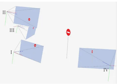
We set up two scenarios of three perspective images of size1000× 2000pixels and a focal length of1400pixels. A circular disk of 80cmof diameter was placed at a mean distance of 10 meters from the images (cf. Fig. 1). The first scenario was composed of imagesSet1 : (I−III −IV)and the second one images
Set2 : (II−III−IV). The approximate distances between
cameras was4m. The difference between the two sets is that in the former the camera centers are almost on the same plane whereas in the latter the cameraIIwas at a distance of3mfrom the horizontal plane containing the two other cameras. The 3D circular disk was sampled regularly at ten 3D points and projected in each camera. The observations consisted in :
• 2D noisy coordinates of projected sampled points in the
im-ages.
• 3D noisy projection centers of the cameras.
• Rotation matrices of the cameras.
I
III
II
IV
Figure 1: Configuration of data simulation
4.2 Simulation results
(a) Scenario 1
(b) Scenario 2
Figure 2: Ellipsoids of errors (99%) corresponding to the cen-ter and normal for both scenarios. Noise of projection cencen-ter = σpc= 1cm
normal vector and Fig. 4 depicts that for center.
Both diagrams demonstrate that generally the errors are larger in the first scenario than the second for both center and normal vec-tor. This is natural since non aligned cameras provide better 3D intersections. This fact is also confirmed by the estimated error ellipsoids since that of second scenario is smaller than the sec-ond one. This is also visible on Fig 2 for one iteration where a Gaussian error ofσ= 1cmwere added to the projection center of cameras. The effective difference between the estimated pa-rameter and the reference one is always smaller than the largest axis of error ellipsoid (99%). This means that the estimated pre-cision of the network is confirmed by the real prepre-cision measured on control points.
On can understand from this experiment that the second image network is much less sensible to pose errors. It can theoretically lead to10cmof error in 3D for a pose error of4cmwhereas the first image network for the same amount of pose error can lead to60cmof error in 3D. By a simple repositioning of cameras on can improve the precision of the 3D measurement system. On can also understand that the improvement (of using scenario 2 vs scenario 1) is much more significant for estimation of normal vector than that center of the circle.
5 CONCLUSIONS AND PERSPECTIVES
We proposed a new approach for reconstructing circular targets from uncertain multiple-views. Our main contributions are in estimating the uncertainty of 2D ellipse and in formalizing per-spective projection of circle with minimum number of parameters
0 0.1 0.2 0.3 0.4 0.5 0.6 0.7
0.01 0.015 0.02 0.025 0.03 0.035 0.04
distance (m)
sigma of Gaussian error applied to the projection center (m)
Scenario 1: difference Scenario 1: Length of largest error ellipsoid axis Scenario 2: difference Scenario 2: Length of largest error ellipsoid axis
Figure 3: Error induced by random errors of projection center to normal vector.
0 0.02 0.04 0.06 0.08 0.1
0.01 0.015 0.02 0.025 0.03 0.035 0.04
distance (m)
sigma of Gaussian error applied to the projection center (m)
Scenario 1: difference Scenario 1: Length of largest error ellipsoid axis Scenario 2: difference Scenario 2: Length of largest error ellipsoid axis
allowing the propagation of observations’ uncertainty to the pa-rameters.
It can be applied for reconstruction of any circular feature us-ing an unlimited number of images with uncertain calibration. It enables also to estimate the precision and stability of a pho-togrammetric network for measuring circular features. Therefore position of the cameras can be optimized (through an analysis-synthesis schema) in order to improve the 3D precision without multiplying the number of the cameras.
The method should be evaluated on more simulated scenarios. Namely by studying its behavior facing more noises on initial 2D points (used for ellipse fitting) and camera rotation matrix but also with more images in complicated camera configurations. Then we aim at evaluating its performance on real data in recon-struction of circular traffic signs (in the same framework devel-oped for reconstruction of polygonal road signs (Soheilian et al., 2013)) and also in detection and reconstruction of circular pho-togrammetric calibration targets.
More theoretically we aim at adapting the method to handle mul-tiple circular features reconstruction at the same time. In more long term we will integrate the developed method in a bundle adjustment chain enabling use of circular features together with their uncertainties as tie and control points.
References
Arlicot, A., Soheilian, B. and Paparoditis, N., 2009. Circular road sign extraction from street level images using colour, shape and texture database maps. International Archives of Pho-togrammetry, Remote Sensing and Spatial Information Sci-ences 38(Part 3/W4), pp. 205–210.
Bergamasco, F., Albarelli, A., Rodola, E. and Torsello, A., 2011. RUNE-Tag: A high accuracy fiducial marker with strong oc-clusion resilience. Cvpr 2011 pp. 113–120.
Bergamasco, F., Cosmo, L., Albarelli, A. and Torsello, A., 2012. A Robust Multi-camera 3D Ellipse Fitting for Contactless Measurements. 2012 Second International Conference on 3D Imaging, Modeling, Processing, Visualization & Transmission pp. 168–175.
Fitzgibbon, A., Pilu, M. and Fisher, R., 1999. Direct least square fitting of ellipses. IEEE Transactions on Pattern Analysis and Machine Intelligence, 21(5), pp. 476–480.
F¨orstner, W., 2005. Uncertainty and projective geometry. In: Handbook of Geometric Computing, Springer, pp. 493–534.
Fu, M. and Huang, Y., 2010. A survey of traffic sign recognition. In: Wavelet Analysis and Pattern Recognition (ICWAPR), 2010 International Conference on, IEEE, pp. 119–124.
Hartley, R. I. and Zisserman, A., 2004. Multiple View Geometry in Computer Vision. Second edn, Cambridge University Press, ISBN: 0521540518.
Heikkila, J., 2000. Geometric camera calibration using circu-lar control points. Pattern Analysis and Machine Intelligence, IEEE pp. 1–29.
Hu, R. and Ji, Q., 2001. Camera self-calibration from el-lipse correspondences. Proceedings 2001 ICRA. IEEE In-ternational Conference on Robotics and Automation (Cat. No.01CH37164) 3, pp. 2191–2196.
Hutter, M. and Brewer, N., 2009. Matching 2-D ellipses to 3-D circles with application to vehicle pose identification. 2009 24th International Conference Image and Vision Computing New Zealand pp. 153–158.
Ip, H. H. and Chen, Y., 2005. Planar rectification by solving the intersection of two circles under 2D homography. Pattern Recognition 38(7), pp. 1117–1120.
Kanatani, K. and Ohta, N., 2004. Automatic detection of circular objects by ellipse growing. International Journal of Image and Graphics 04(01), pp. 35–50.
Mai, F., Hung, Y. S. and Chesi, G., 2010. Projective reconstruc-tion of ellipses from multiple images. Pattern Recognition 43(3), pp. 545–556.
Martelli, S., Marzotto, R., Colombari, A. and Murino, V., 2010. Fpga-based robust ellipse estimation for circular road sign de-tection. In: Computer Vision and Pattern Recognition Work-shops (CVPRW), 2010 IEEE Computer Society Conference on, pp. 53–60.
Mateos, G., 2000. A camera calibration technique using targets of circular features. Department of Computer Science and Sys-tems, . . . .
McGlone, J. C., Mikhail, E. M. and Bethel, J. S., 2004. Manual of Photogrammetry. 5th eddition edn, American Society of Photogrammetry and Remote Sensing.
Quan, L., 1996. Conic reconstruction and correspondence from two views. IEEE Transactions on Pattern Analysis and Ma-chine Intelligence 18(2), pp. 1–13.
Ravanbakhsh, M. and Fraser, C., 2009. Road Roundabout Extrac-tion From Very High ResoluExtrac-tion Aerial Imagery. Proc. CMRT XXXVIII, pp. 3–4.
S. Ji, Y. S. and Shi, Z., 2012. Manhole Cover Detection using Vehicle-based Multi-Sensor Data. International Archives of the Photogrammetry, Remote Sensing and Spatial Information Sciences XXXIX-B3(September), pp. 281–284.
Shuhua, L. and Yong, T., 2010. A robust high-precision circular target detection method based on hough transform. In: Com-puter Application and System Modeling (ICCASM), 2010 In-ternational Conference on, Vol. 14, pp. V14–253–V14–257.
Soheilian, B., Paparoditis, N. and Vallet, B., 2013. Detection and 3d reconstruction of traffic signs from multiple view color im-ages. ISPRS Journal of Photogrammetry and Remote Sensing 77, pp. 1 – 20.
Tarel, J.-P. and Gagalowicz, A., 1995. Calibration de cam´era `a base d’ellipses. Traitement du Signal 12(2), pp. 177–187.