THE POTENTIAL OF LOW-COST RPAS FOR MULTI-VIEW RECONSTRUCTION OF
SUB-VERTICAL ROCK FACES
K. Thoeni a, D.E. Guccione b, M. Santise b, A. Giacomini a, R. Roncella b, *, G. Forlani b
a Centre for Geotechnical and Materials Modelling, The University of Newcastle, Callaghan, NSW 2308, Australia (klaus.thoeni, anna.giacomini)@newcastle.edu.au
b Department of Civil, Environmental, Land Management Engineering and Architecture, University of Parma, via Parco Area delle Scienze, 181/a, 43124 Parma, Italy
(davideettore.guccione, marina.santise)@studenti.unipr.it, (riccardo.roncella, gianfranco.forlani)@unipr.it
Commission V, WG V/5
KEY WORDS: UAV, Close Range Photogrammetry, Structure from Motion, Action Camera, Calibration, Accuracy, Coded Targets, Natural Features
ABSTRACT:
The current work investigates the potential of two low-cost off-the-shelf quadcopters for multi-view reconstruction of sub-vertical rock faces. The two platforms used are a DJI Phantom 1 equipped with a Gopro Hero 3+ Black and a DJI Phantom 3 Professional with integrated camera. The study area is a small sub-vertical rock face. Several flights were performed with both cameras set in time-lapse mode. Hence, images were taken automatically but the flights were performed manually as the investigated rock face is very irregular which required manual adjustment of the yaw and roll for optimal coverage. The digital images were processed with commercial SfM software packages. Several processing settings were investigated in order to find out the one providing the most accurate 3D reconstruction of the rock face. To this aim, all 3D models produced with both platforms are compared to a point cloud obtained with a terrestrial laser scanner. Firstly, the difference between the use of coded ground control targets and the use of natural features was studied. Coded targets generally provide the best accuracy, but they need to be placed on the surface, which is not always possible, as sub-vertical rock faces are not easily accessible. Nevertheless, natural features can provide a good alternative if wisely chosen as shown in this work. Secondly, the influence of using fixed interior orientation parameters or self-calibration was investigated. The results show that, in the case of the used sensors and camera networks, self-calibration provides better results. To support such empirical finding, a numerical investigation using a Monte Carlo simulation was performed.
* Corresponding author
1. INTRODUCTION
RPAS, also known as drones or UAVs, have been used in military applications for many years. Nevertheless, the technology has become accessible to everyone only in recent years. Electric multirotor helicopters or multicopters have become one of the most exciting developments, and several off-the-shelf platforms are now available. Multicopters allow for both horizontal and vertical photogrammetric strips in close proximity to the object of interest. Together with the recent advances in photogrammetry through the application of Computer Vision (CV) techniques (Hartley & Zisserman, 2003) such platforms are becoming more and more popular among scientists and professionals (Bolognesi et al., 2015; Arango & Morales, 2015). Indeed, RPAS photogrammetry introduces a low-cost alternative to classical manned aerial surveys for topographic mapping and detailed 3D reconstruction of ground information (Nex and Remondino, 2014). In addition, changing regulations, such as the one in Australia where by the end of this year everyone will be allowed to operate RPAS with mass less than 2 kg without a specific license, make such platforms even more attractive. Nevertheless, it is still not clear how such platforms can be used most efficiently to get the required accuracy for photogrammetric surveys. There is still a need to
develop simple guidelines for the use of low-cost RPAS surveys in order to obtain accurate and reliable results.
precision agriculture (Fritz et al., 2013). However, platforms weighting over 2 kg are not generally low-cost. They also carry DSLR or compact cameras with stable optics and reasonable good image sensors. Low-cost platforms, instead, come with light-weight cameras with optics made of plastic and sensors using a rolling shutter (Chabok, 2013). Hence, they are generally not suitable for accurate photogrammetric surveys. Nevertheless, the trend shows that such cameras are getting better and commercial photogrammetry packages start to overcome the problems such optics and sensors introduce. In this context, reliable camera calibration procedures and a good understanding and implementation of efficient image network geometry are essential to provide good results and to partly overcome the lower optic quality (Harwin et al., 2015). Typical image-based RPAS surveys require a flight plan and ground control points (GCPs) (Nex and Remondino, 2014). A flight plan is useful to ensure the required overlap of the images and to define the camera network. However, it strongly relies on the on-board navigation system (e.g., GPS) which might not be accurate and usually relies as well on available maps. Hence, rigorous flight planning is not always possible, especially when working at the close proximity of very small and complex or even vertical object. In fact, the main focus on RPAS photogrammetry has been on horizontal surveys for which flight plans can easily be created and GCPs are available. GCPs are needed for accurate georeferencing and as well to improve the overall accuracy of the model (e.g., minimisation of systematic errors). The accuracy of the final product depends not only on the accuracy of the GCPs coordinates (which should be higher than the accuracy requirements of the final survey) but as well on the accuracy by which control points are detected and marked on the images (Caroti et al., 2015). Hence, coded targets are preferred, as they are generally detected automatically. However, in many cases it is not feasible to apply coded targets on the object to be surveyed because the object itself cannot be accessed. In such cases, natural features on the object are generally used as control points. Since the operator has to manually mark these points they must be high visibility and easy to find in the images.
The current paper investigates the potential of low-cost multicopters, such as the DJI Phantom, for the 3D mapping of sub-vertical rock faces and aims to develop some simple guidelines for the use of low-cost RPAS surveys in order to obtain accurate 3D models. The images were processed using the two commercial SfM software packages Agisoft Photoscan Professional and Pix4D Mapper Pro. Firstly, the influence between the use of coded ground control targets and natural features was investigated. Coded targets provide the best accuracy, but they need to be placed on the surface, which is generally not possible on sub-vertical rock faces. Secondly, the influence of using fixed interior orientation parameters (i.e., static pre-calibration) or self-calibration (i.e., computing a single parameter set for the whole sequence or an individual set for each image) was investigated in detail. Finally, a numerical investigation using a Monte Carlo simulation was developed to support the findings.
2. METODOLOGY
2.1 RPAS platforms and cameras
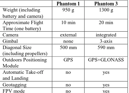
The platforms used are two low-cost off-the-shelf quadcopters produced by the same company. The first is a DJI Phantom 1 (P1) equipped with a Gopro Hero 3+ Black Edition and the
second is a DJI Phantom 3 Professional (P3) with integrated camera. Both platforms cost less than 1500 € including the camera. Figure 1 shows both platforms side by side. The P1 was released in early 2013 and was the first reliable low-cost quadcopter on the market. It comes with a GoPro mount and the total weight including camera is less than 1 kg.
Figure 1. Phantom 1 with GoPro 3+ Black (left) and Phantom 3 Professional with integrated camera and 3-axis gimbal (right).
In April 2015 DJI released the P3 with major improvements compared to the P1. A higher capacity battery and bigger propellers allow for an increase of the flight time by a factor of two. A newly developed visual positioning system allows for automatic take-off and landing and for hovering without GPS. In addition, the positioning module integrates GPS and GLONASS. All these improvements allow for a more stable flight. Finally, the P3 includes an integrated camera mounted on a 3-axis gimbal which is attached to the body of the quadcopter by four damping elements. The output of the camera can be
Table 1. Main characteristics of the RPAS used during the test.
GoPro 3+ Black (P1)
Sony EXMOR (P3) Image Sensor Size 1/2.3" 1/2.3" Pixel Resolution 3000x4000 3000x4000
Pixel Size 1.55 μm 1.55 μm
Table 2 lists the main characteristics of the cameras used. Both cameras have the same image sensor with a resolution of 12MP and a fixed focal length. The main differences are that the GoPro has a fisheye lens and hence a bigger field of view (FOV) but the image is as well more distorted compared to the one of the P3. In addition, the time-lapse mode of the GoPro allows for much smaller time intervals. It should also be mentioned that the GoPro Hero 3+ Black Edition comes with FPV functionality. However, it uses the same transmission frequency as the remote control of the P1 and interferes with it which could result into an uncontrolled crash. Hence, this functionality should not be used.
2.2 Area of study
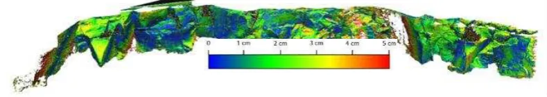
The area of study is a small sub-vertical rock face in Pilkington Street Reserve in Newcastle (NSW, Australia), near the Callaghan Campus of the University of Newcastle. The area is part of an abandoned sandstone quarry and is currently used as recreation area. Being a dismissed mining facility, the study site represents an exemplar case for applicative purposes but, at the same time, does not present the strict accessibility constraints of a working quarry, allowing the authors to perform all the survey operation in a safer and simpler environment. The rock wall under investigation is partly smooth with some evident geological features such as non-persistent joints and sharp edges (Thoeni et al., 2014). It is as well irregular and curved in the horizontal direction. The rock face has a distinctive texture with many colours and natural features (e.g., natural spots and marks of lichen). The view towards the wall is free from bushes and trees and there is enough space for smooth and safe operations of the quadcopters. An overview of the investigated rock face is shown in Figure 2. The considered part of the wall is about 80 m long and has an average height of about 6 m.
2.3 Field work and data acquisition
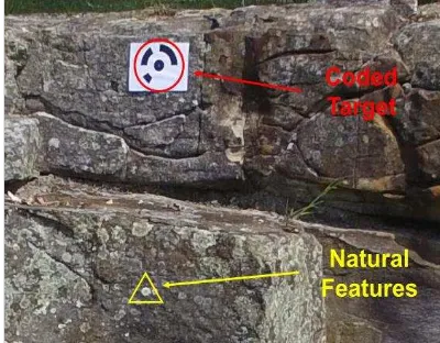
The first step in the field was to place coded control point markers on the wall. A total of 18 coded targets were attached to the rock face by walking at the base and top of the wall and by using a stepladder. Figure 2 shows their location on the wall with a red circle. After setting them up, their coordinates where measured by using two Leica TS11 reflectorless total stations. In order to improve the accuracy, the measurements were taken from two different positions.
The second step consisted in selecting and measuring a set of well distributed and easy-to-find natural features. This was not a trivial task and a special procedure was adapted. All natural features were chosen very carefully since it is very important to be able to exactly locate the points in the aerial images. To assist with this process, additional close-up pictures where taken with a digital camera with a zoom lens. The camera was set up on a tripod and the pictures were taken by activating the grid on the LCD display which allowed having the feature exactly in the centre of the image. In addition, a picture with a tablet was taken and notes were directly written on the picture. Other important aspects which were considered for the selection
of a natural feature were its immediate surroundings. In contrast to coded targets, natural features are generally not recognised automatically by the processing software and need to be selected manually by the operator on at least a couple of images. Hence, natural features should be away from sharp edges or holes in order to avoid the risk of selecting points which are almost the same on the image but have different spatial coordinates. A similar problem arises when measuring the points with the two total stations. Therefore, the measurements were taken simultaneously by the same operator after double-checking the readings on both instruments. Figure 3 shows a close-up view of the natural features and coded targets used. A total of 13 natural targets were measured.
Figure 3. Example of coded target and natural feature.
The third and final step involved flying the RPAS and taking pictures of the wall. Because of the significant irregularity of the rock surface, an adjustment of the yaw and roll (only possible on P3) was required to reach an optimal coverage. Therefore, all flights were conducted manually and very close to the object maintaining a constant distance from the wall during the flight.
Two main flight patterns were adjusted for maximising the overlap: horizontal and vertical strips for combined nadir and oblique image capture. The goal was a ground sampling distance (GSD) of less than 5 mm/pixel. Hence, the required distance of the flight path from the wall needed to be below 10 m. During the acquisition, an overlap and a sidelap of at least 80% between adjacent images was reached. Since the P1 has no FPV capabilities and is much more unstable in the air compared to the P3, the time interval for the time-lapse on the GoPro was set to the minimum 0.5 s. This resulted in a huge amount of images, which was reduced before processing. The time-lapse on the P3 was set to the minimum 5 s. A continuous flight path with very low velocity was adapted for the P1 whereas a stop-go approach was adapted for the P3, since the time interval was much bigger. The P3 allowed also the adjustment of the camera roll during the flight. The FPV mode was a great help during the flight since it allowed estimating how close the quadcopter is to the wall more easily.
In order to limit processing time and allow for a fair comparison between the two platforms a similar number of images was selected. The initial survey with the P1 resulted in almost 2000 images. This number was first reduced by just taking every fifth (this corresponds to a time interval of 2.5 s). Then the image quality was estimated in Photoscan and all images with a quality lower than 0.8 where disregarded. The final number of images for the P1 and the P3 was 254 and 296 respectively.
2.4 Reference model
The ground truth or reference model was created using a Leica ScanStation C10 terrestrial laser scanner (TLS) with a range accuracy of ±4 mm. The TLS automatically provides the user with dense 3D point clouds. Three scans from three different locations were undertaken in order to improve the accuracy and minimise occlusions. The corresponding point clouds were stitched together using the known locations of the stations and other features within the scene. The scan processing software Leica Cyclone was used for this purpose. Noise, outliers and duplicated points were automatically detected and removed.
3. DATA PROCESSING
3.1 Multi-view 3D reconstruction
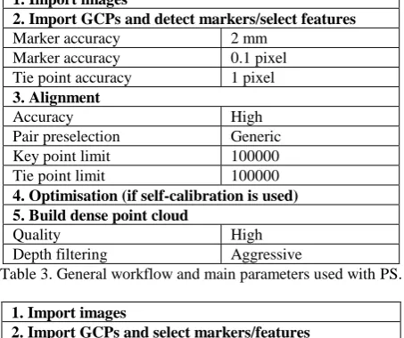
The digital images were processed with the two commercial SfM software packages Agisoft Photoscan Professional (PS) and Pix4D Mapper Pro (Pix4D). Both packages are very user-friendly and have an almost automated photogrammetric workflow. Tables 3-4 show the general workflow with the most relevant processing parameters.
1. Import images
2. Import GCPs and detect markers/select features
Marker accuracy 2 mm
Table 3. General workflow and main parameters used with PS.
1. Import images
Table 4. General workflow and main parameters used with Pix4D.
The workflow of both packages is very similar. However, the coded targets were detected automatically by PS only. The detection (detect marker function) worked correctly for the images collected by the P3. Instead, difficulties were encountered for the P1 fish-eye imagery, with only 10 of the 18 targets identified automatically. Hence, the remaining 8 where collimated manually. In Pix4D, both coded targets and natural features needed to be detected manually by the operator. Nevertheless, the Pix4D workflow integrates an additional step for automarking of GCPs and checking their collimation error. This advanced feature can be very useful especially when natural features are being used.
3.2 Camera calibration
One of the most critical stages in the photogrammetric workflow of a low-cost RPAS survey is the camera calibration. The quality of the cameras and optics usually implemented in principal interior orientation and distortion parameter in different surveys (and, sometimes, also in the context of the same survey) should be expected. On the other hand, providing an ad-hoc camera calibration procedure is the best and more reliable solution to prevent unwanted parameter correlations and biases.
This work investigates the influence of the camera calibration in the digital surface model (DSM) restitution considering three different calibration methods: a traditional test field calibration (TFC) and two self-calibration methods, called hereafter Single-Camera calibration (SCS) and Multi-Single-Camera Self-calibration (MCS).
In the TFC, suitable coded target points, with known coordinates, are captured from several camera stations with convergent (oblique) images (Clarke & Fryer, 1998). It is important, as far as possible, that the object points do not lie on the same object plane and that at least some cameras are tilted around their optical axis of approximately 90 degrees. This limits unwanted correlations between the estimated parameters (in particular between principal distance and principal point location with exterior orientation parameters).
SCS and MCS estimate the interior orientation and distortion parameters using the very same images acquired for the actual survey of the object. In SCS a single set of parameters, identical for all the images, is estimated. In MCS several sub-set of images, each one with its individual set of camera model parameters, are estimated. MCS can be useful in low-cost RPAS surveys, where lack of camera or optics stability should be expected. However, the method can amplify parameter correlation and the numerical instability of the bundle-block if the image block is not rigid and sufficiently redundant.
In this work, a TFC was performed using a temporary test field, realized at the University of Newcastle (Australia) in the local rugby field (see Figure 4) where 25 blocks, each with 5 coded targets, were materialized on rigid panels and imaged using the P1 and P3. The acquisition of the image sequence required a good level of piloting skill and carefulness, in order to provide an optimal imaging geometry. The calibration parameters have been estimated with Photomodeler Scanner.
included in the self-calibrating Bundle Block Adjustment (BBA) (Harwin et al., 2015). SCS and MCS are implemented as processing options in both environments. The MCS method was applied in the experiment with an individual set of camera model parameters for each image.
Figure 4. Field calibration: P1 (left) and P3 (right).
3.3 Data analysis
The pipeline of Table 3 and 4 were carried out using the same set of RPAS-based images with all estimated sets of calibration parameters. The aim was to verify the effectiveness of different control points (coded and natural targets) and identify the influence of different calibration methods on the accuracy of the generated DSM. Two different comparisons were conducted to verify the quality of the different blocks. Firstly, the BBA was verified using check points (CP). In the case of the coded targets 9 points were used as GCP and the remaining 9 as CP. In the case of the natural features all coded targets served as CP. Secondly, the overall accuracy of the models was assessed by comparing the DSMs to the reference model of the TLS using the open-source software CloudCompare.
4. RESULTS AND DISCUSSION
4.1 Target vs. Natural features
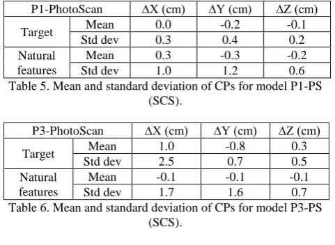
SCS is used for the comparisons conducted using different GCPs. The CP comparison has only been carried out with the models generated with PS (Tables 5-6). While with P1 coded targets provided a better accuracy, this was not the case for P3.
P1-PhotoScan ∆X (cm) ∆Y (cm) ∆Z (cm)
Target Mean 0.0 -0.2 -0.1
Std dev 0.3 0.4 0.2
Natural features
Mean 0.3 -0.3 -0.2
Std dev 1.0 1.2 0.6
Table 5. Mean and standard deviation of CPs for model P1-PS (SCS).
P3-PhotoScan ∆X (cm) ∆Y (cm) ∆Z (cm)
Target Mean 1.0 -0.8 0.3
Std dev 2.5 0.7 0.5
Natural features
Mean -0.1 -0.1 -0.1
Std dev 1.7 1.6 0.7
Table 6. Mean and standard deviation of CPs for model P3-PS (SCS).
The comparison of the DSMs with the reference model was performed including as well the results of Pix4D. The standard deviations of the differences after the alignment were similar, equal to 0.9 cm, independently of the GCP used. Improved accuracy was observed for the P3 models generated by Pix4D, with a standard deviation equal to 0.6÷0.7 cm.
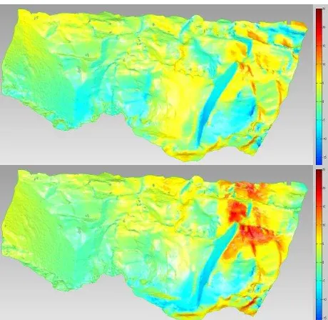
The analysis of the distance maps for the entire model showed that different configurations of bundle block adjustments
produce significant local deformation in the distance maps (Figures 5a-b). This effect was again less evident on the model generated using Pix4D. This could be attributed to its automarking tool. To the contrary, PS needs manual collimation of natural features, used as GCPs, that produces bigger errors and local deformations, as shown in Figure 6.
Figure 5. Error mapping of the deviation between: (a) TSL and model P3-PS-Target and (b) TSL and model P3-PS-Natural
features.
Finally, using natural features or coded targets does not affect significantly the accuracy of the block orientation and the DSM generation. However, considering the image scale and the GSD, if coded targets provide reliable data for the block orientation, an incorrect identification of the natural features and their collimation could introduce significant local deformation.
4.2 TFC, SCS and MCS calibration tests
A traditional TFC calibration provides reliable results. However, the use of RPAS platforms with low-cost digital cameras could provide non-negligible variations of the interior orientation and distortion parameters during take-off, flight and landing operations. This was clearly highlighted in the present work: the bundle adjustment showed residuals on CP within the 2.4÷3.2 cm range (unlike the 0.5÷1.0 cm range obtained with SCS) and a standard deviation of the differences between the photogrammetric and the reference DSMs of 2.2 cm only, compared to the 0.6÷1.0 cm measured with the SCS. Figure 6 shows systematic deformations of the DSM over the entire model above 5cm (10 times the GSD). The errors on CP of SCS and MCS show comparable values: 0.5-1.0 cm RMSE for most of the models of P1. Similarly, the comparison with the TLS model gave RMSE of 0.8÷0.9 cm. However, local differences can be observed in the two different calibration methods (Figure 7). In particular, more significant local deformations extended over the entire model were observed in the case of the natural features identification with the MCS model (Figure 8).
4.2.1 SCS vs MCS comparison
The results obtained using MCS calibration, showed that in most of the cases, although the degree of freedom of the BBA might be alarming (if its redundancy and stability is not good enough) the results are as satisfactory as the corresponding SCS test. In the test depicted in Figure 7a, localised deformation of the DSM (and consequently, with high probability, of the corresponding section of the image block) are evident in two different areas. In the left area of the DSM, indicated with (A), the MCS solution presents deviations up to ca. 1 cm. In the corresponding image block subset, a much higher variability of the camera model parameters was found, far beyond the reasonable variability expected in the test conditions. A plausible justification for this is that the higher degree of freedom of the bundle block system, if not supported with enough good ray-intersection observations and a good imaging
(a)
geometry, would lead to an unstable exterior orientation parameter estimation that systematically introduces shape deformation in the DSM. On the other hand, in the right part of the DSM (indicated in Figure 7b with the letter (B)) it is worth noting that, while all the SCS tests provided significantly worse results than in the other areas of the model, with mean differences of more than 2 cm, the MCS showed always good performances.
Moreover, the differences with the reference model are much more evident on all the surfaces facing rightward, while in the areas parallel to the mean slope direction, the differences are more similar to those observed in the other parts of the digital model. That would probably suggest that such discrepancies are not necessarily connected with the imaging geometry (if that would be the case, MCS should have done much worse than SCS), but, more likely, depend on some kind of bias, being a wrong GCP the main suspect. The more adaptable MCS bundle block adjustment, in conjunction with a huge rigidity of the block (many tie points, whose total number is ca. 300000, are imaged in more than 50 frames), would probably absorb the bias faster than SCS, limiting its influence only in the neighbourhood of the GCP itself. To test the feasibility of such hypothesis (wrong GCP identification), a numerical simulation by means of a Monte Carlo (MC) simulation was set up to model the effective behaviour of the two self-calibration procedures.
4.2.2 Monte Carlo simulation
To run the simulations, an ad-hoc .NET experimental MC framework was developed. The image block geometry is specified using a fairly simple and intuitive configuration file where the user can describe the block structure. Different object shapes can be defined procedurally or using a discrete set of 3D points: in this case a set of 30000 object points uniformly distributed on the rightmost part of the DSM were used. A subset of 700 points was considered for the generation of the tie-points, trying to reproduce the actual image point distribution of the real-case photogrammetric block, both in terms of redundancy and frame occupancy. The points are projected on the available image frames (a subset of 110 images with the same exterior and interior orientation parameters of the real image block) and used as tie-points, using a pseudo-random assignment algorithm to the images themselves. If, on one hand, it is unrealistic that every ground point is recognised by the interest operator in every image framing the point itself, on the other, a lower multiplicity limit (points are visible on many images considering the great overlap of adjacent frames) should be enforced. The user, therefore, specifies a lower and upper limit for point multiplicity and the algorithm produces a random assignment of the tie-point, avoiding configuration with unlikely distributions (e.g., base length too small or too wide). For all the simulations, 7 GCPs on the boundary of the DSM portion were used, one of which, in the upper-rightmost area of Figure 6. Error mapping of deviation between TSL and model P3-PS-Target-TFC.
Figure 7. Error mapping of the deviation between (a) TSL and model MCS and (b) TSL and model P3-PS-Target-SCS.
Figure 8. Error mapping of deviation between TSL and model P3-PS-Natural-MCS. (a)
the DSM, was given a systematic error of 3 cm along a direction parallel to the slope front.
Finally, the procedure to be used during the BBA (e.g., SCS or MCS) is specified by the user. It is worth noting that, during tie point projection (error free) the same camera model parameter set was used: the augmented degree of freedom provided by MCS is not necessary, since the error-free solution should provide the same parameters for all the cameras.
A routine performs the MC simulations iterating the bundle adjustment procedure and collecting the orientation solution and the estimated object structure (coordinates of tie-points) at the end of each iteration. The MC framework can be interfaced with several BBA routines. In particular, the CALGE BBA module (Forlani & Pinto, 1994), a widely tested scientific package, was considered the most versatile and efficient for the different case studies.
In a second stage all the object points are triangulated with the parameters coming from the BBA, and compared with the original points of known coordinates. The comparisons presented in the previous section considered the minimum distance between the two surfaces represented by the reference TLS survey and the photogrammetric reconstructed DSM. Hence, the distances between known and calculated object points are projected on the local DSM normal vector.
To summarise the entire simulation workflow:
(i) in a first stage the pseudo-random algorithm assigns tie-points, on the basis of 700 uniformly distributed ground tie-points, to the different images considering the lower (10) and upper (20) limit specified by the user;
(ii) the 7 GCP (without errors) are projected on all the available images;
(iii) all image coordinates are summed with a random normal error (σ = 0.5 pixel);
(iv) the upper-rightmost GCP object coordinates are changed systematically, moving the points 3 cm in a horizontal direction parallel to the slope front;
(v) the observation system (more than 20k observations) is solved using the CALGE BBA considering a SCS or MCS on-the-job calibration routine. At this point the interior and exterior orientation parameters are output and assigned to a new block where a higher number of tie-points are considered:
(vi) the output of the BBA solution is read;
(vii) the set of 30k object points uniformly distributed on the DSM portion are projected and assigned as tie-points to the images;
(viii) all image coordinates are summed with a random normal error (σ = 0.5 pixel);
(ix) a least square triangulation procedure computes the corresponding object point coordinates;
(x) the distance between each initial and computed object point along the DSM local surface normal is calculated and stored.
The entire procedure (step (i) to (x)) has been iterated 2000 times. The results of the two simulations, the first considering the SCS calibration procedure, the second the MCS calibration, are presented in Figure 9.
Indeed, as far as the surfaces facing toward the right side of the DSM are concerned, the MCS solution provides better results, with systematic deformed areas much smaller and with lower values. The effect of the GCP bias disappears in the central and leftmost areas of the selected region. On the other hand, the red areas depicted in the upper-right area of the DSM (most of the surface faces towards the observer) are much larger for MCS than SCS.
Figure 9. MC simulation comparison: SCS calibration solution (top); MCS calibration solution (bottom).
It is worth noting, however, that in this area the redundancy of the observations is much lower than in the rest of the block, since near the block edges less images overlap. In this area, it is likely that higher degree of freedom of the MCS makes the emergence of the image block/DSM localised deformation easier.
Although the two MC simulation cannot be considered exhaustive, some interesting points, to be further investigated, have emerged. The use of MCS calibration should be discouraged, in particular if the redundancy does not guarantee the stability of the solution all over the block. On the other hand, if the block is sufficiently rigid and self-consistent, MCS allows the internal coherence of tie-point observations to reduce systematic deformation due to gross errors coming standard deviation.
5. CONCLUSIONS
The paper presented a series of metric comparison considering RPAS survey of sub-vertical rock faces, using low-cost platforms and commercial SfM software packages. It has been shown that, with proper ground control and high overlaps, accuracies fully comparable to TLS can be obtained. Most likely, the progressive deregulation of RPAS flight operations in the near future will greatly increase the application scope of these systems. At the same time, the progress in automatic image orientation and surface reconstruction has made available easy-to-use, turnkey software that is making photogrammetry increasingly appealing also to untrained or inexperienced users. The documentation of the results provided by these programs is often lacking in details, giving the feeling that everything is always right.
Finally, if natural features are used as GCP they should be chosen wisely and double checked by two or more measurements.
ACKNOWLEDGEMENTS
The authors would like to gratefully acknowledge the assistance provided by Michele Spadari and Ronald Murtagh during data collection. In addition, the authors would like to acknowledge the financial support of the University of Newcastle (ECR Grant G1300601) and the Australian Coal Association Research Program (ACARP C23026).
REFERENCES
Achille, C., Adami, A., Chiarini, S., Cremonesi, S., Fassi, F., Fregonese, L., & Taffurelli, L., 2015. UAV-Based Photogrammetry and Integrated Technologies for Architectural Applications – Methodological Strategies for the After-Quake Survey of Vertical Structures in Mantua (Italy). Sensors, 15(7), pp. 15520-15539.
Agisoft PhotoScan Professional (version 1.2.0.2198),
http://www.agisoft.com (9 April 2016).
Arango, C., & Morales, C. A., 2015. Comparison between multicopter UAV and total station for estimating stockpile volumes. ISPRS International Archives of the Photogrammetry, Remote Sensing and Spatial Information Sciences, XL-1/W4, pp. 131-135.
Bolognesi, M., Furini, A., Russo, V., Pellegrinelli, A., & Russo, P., 2015. Testing the low-cost RPAS potential in 3D cultural heritage reconstruction. ISPRS International Archives of the Photogrammetry, Remote Sensing and Spatial Information Sciences, XL-5/W4, pp. 229–235.
Caroti, G., Martínez-Espejo Zaragoza, I., & Piemonte, A., 2015. Accuracy assessment in structure from motion 3D reconstruction from UAV-born images: the influence of the data processing methods. ISPRS International Archives of the Photogrammetry, Remote Sensing and Spatial Information Sciences, XL-1/W4, pp. 103-109.
Chabok, M., 2013. Eliminating and modelling non-metric camera sensor distortions caused by sidewise and forward motion of the UAV. In: Proceedings of the International Conference on Unmanned Aerial Vehicle in Geomatics, pp. 73-79.
Clarke, T. A., & Fryer, J. G., 1998. The development of camera calibration methods and models. The Photogrammetric Record, 16(91), pp. 51-66.
CloudCompare (version 2.6.2), http://www.danielgm.net/cc (9 April 2016).
Forlani, G., & Pinto, L., 1994. Experiences of combined block adjustment with GPS data. In: Spatial Information from Digital Photogrammetry and Computer Vision: ISPRS Commission III Symposium, pp. 219-226.
Hallermann, N., Morgenthal, G., & Rodehorst, V., 2015. Vision-based monitoring of heritage monuments – Unmanned Aerial Systems (UAS) for detailed inspection and high-accurate survey of structures'. In: Proceedings of STREMAH, pp. 621-632.
Hartley, R., & Zisserman, A., 2003. Multiple view geometry in computer vision. Cambridge University Press.
Harwin, S., Lucieer, A., & Osborn, J., 2015. The Impact of the Calibration Method on the Accuracy of Point Clouds Derived Using Unmanned Aerial Vehicle Multi-View Stereopsis. Remote Sensing, 7(9), pp. 11933-11953.
Morgenthal, G., & Hallermann, N., 2014. Quality assessment of Unmanned Aerial Vehicle (UAV) based visual inspection of structures. Advances in Structural Engineering, 17(3), pp. 289-302.
Nex, F., & Remondino, F., 2014. “UAV for 3D mapping applications: a review”. Applied Geomatics, 6, pp. 1-15.
PhotoModeler Scanner (version 2012.2.1.779),
http://www.photomodeler.com (9 April 2016).
Pix4D Mapper Pro (version 2.0.104) https://www.pix4d.com (9 April 2016).
Reich, M., Wiggenhagen, M., & Muhle, D., 2012. Filling the holes–Potential of UAV-based photogrammetric façade modelling. In Tagungsband des 15. 3D-NordOst Workshops der GFat, pp. 147-156.
Thoeni, K., Giacomini, A., Murtagh, R., & Kniest, E., 2014. A comparison of multi-view 3D reconstruction of a rock wall using several cameras and a laser scanner. ISPRS International Archives of the Photogrammetry, Remote Sensing and Spatial Information Sciences, XL-5, pp. 573-580.