Modelling global radiation in complex terrain: comparing
two statistical approaches
Helfried Scheifinger
a,∗, Helga Kromp-Kolb
baCentral Institute for Meteorology and Geodynamics, Hohe Warte 38, A – 1190 Vienna, Austria bInstitute for Meteorology and Physics, University of Agriculture, Türkenschanzstraße 18, A – 1180 Vienna, Austria
Received 1 June 1999; received in revised form 27 September 1999; accepted 7 October 1999
Abstract
Two simple approaches for assessing global radiation in complex terrain are tested and compared. A parameterisation scheme for global radiation based on cloud cover observations was compared with interpolation of measured global radiation values from the Austrian climate observation network. Interpolation appears to be a useful method for a station density which has been available after 1992 in Austria (about 1000 km2/station). In that case interpolation is superior to parameterisation.
The quality of interpolated data quickly drops with height and for elevations above 1500 m neither method delivers useful results. ©2000 Elsevier Science B.V. All rights reserved.
Keywords: Global radiation; Atmospheric transmittance; Parameterisation; Interpolation; Complex terrain
1. Introduction
The atmospheric environment constitutes a deci-sive factor controlling ecosystem processes. Most pro-cesses in the atmosphere and biosphere, such as evap-oration, sensible heat flux, soil heat flux, photosynthe-sis or transpiration, are driven directly or indirectly by solar radiation. Many of them have been investigated and modelled in recent years by various disciplines not only in flat but also in complex terrain, where so-lar radiation constitutes a basic input.
In order to investigate and quantify possible rela-tions between temporal and spatial distriburela-tions of ecosystem and atmospheric variables in complex ter-rain, the temporal and spatial resolution of both
vari-∗Corresponding author. Tel.:+43-1-36026; fax:+43-1-36026-74.
E-mail address: [email protected] (H. Scheifinger).
able sets must match. Because of the high spatial vari-ability of ecosystems in complex terrain, atmospheric information with a high spatial resolution is often seen as a prerequisite for ecological research there. Some-times it is not easy to acquire the atmospheric data with the necessary spatial resolution in remote areas. Putting up and running a fully instrumented meteo-rological station can be costly. Points of investigation can be spread across a huge area, and not at each of them all atmospheric variables can be measured. If the measurement of only a selected set of atmospheric variables can be afforded, information about others which are also important, might be still lacking. In such situations one has to look for other sources of information:
1. Luckily most countries are running meteorological networks, which provide information about the at-mospheric environment to be utilised. A straight-forward solution would be to extrapolate and use
the data from the nearest meteorological station. Because of the horizontal and vertical distance be-tween the meteorological station and the place of interest, such a procedure can be dangerous and can deliver unsatisfying results. Unfortunately ecosys-tem research focuses often on such remote places where data are scarce. National climate observation networks have not been designed to supply data with a high spatial resolution in remote alpine ar-eas. The more one moves from flat and inhabited areas to remote and complex terrain the more sta-tion density drops. Stasta-tion density is also rapidly decreasing with increasing height.
2. In many cases a strong relationship between the desired atmospheric variable and topogra-phy can be found. Topographical information can be available more readily and with a much higher spatial resolution than for any atmospheric variable.
3. A third source of information can be found in the observation that atmospheric variables do not behave independently. One would have to select proper independent atmospheric variables which allow a tight relationship with the desired depen-dent variable. In case the independepen-dent atmospheric variable is measured with a higher spatial density than the dependent variable, additional spatial in-formation for the dependent atmospheric variable can be deduced. Where radiation is concerned, sunshine duration, cloudiness, degree hours of temperature, relative humidity, precipitable wa-ter content, and composition, concentration and size distribution of aerosols are among the in-dependent variables which have been used for parameterisation. The usefulness of a parameteri-sation scheme depends very much on the spatial behaviour of the chosen variables. Some authors, for instance, selected temperature and precipita-tion as independent variables which can cause problems, if applied in complex terrain. The pa-rameterisation schemes might work at the few places where they were developed for but not necessarily at other sites. In order to apply a pa-rameterisation scheme as it was developed by Bristow and Campbell (1984) or Lexer (1997), empirical coefficients would have to be interpo-lated in complex terrain. As the spatial behaviour of temperature and precipitation in complex
terrain is as complex as the terrain, such an approach appears impractical.
4. As a fourth point, general knowledge about the physics of an atmospheric variable can add substan-tial information: laws describing the relative posi-tion of the sun on a tangential plane on the earth’s surface and shading through topographical features as a function of time help to calculate global radi-ation at a specific point in complex terrain. Or the idea of global radiation as a sum of direct radiation, diffuse radiation and radiation reflected from the earth’s surface greatly supports the reconstruction of global radiation from interpolated transmittance values.
This work aims at a straightforward and easily ap-plicable procedure to produce radiation data in com-plex terrain based on the four above mentioned sources of information. Although the procedures which will be introduced show certain limitations, they can nev-ertheless prove their usefulness for a number of appli-cations.
As it was impossible to find a suitable procedure which could solve the stated problems, two approaches were developed and compared. One was the interpo-lation of measured global radiation sums (daily and monthly values) via atmospheric transmittance and the other, a parameterisation scheme with subsequent in-terpolation of the parameterised atmospheric transmit-tances. For parameterisation, cloud cover observations and the height of the cloud observing station were selected as independent parameters.
Comparing advantages and disadvantages of the pa-rameterisation and interpolation approach, following factors have to be considered:
1. Station density for global radiation measurements (more than 1000 km2/station in Austria).
2. Station density for cloud observations (less than 300 km2/station in Austria).
3. Quality loss through parameterisation. 4. Quality loss through interpolation.
2. Radiation in complex terrain
Various gaseous, liquid and solid components of the atmosphere, like ozone, aerosols, water droplets, cloud droplets, and the earth’s land and sea surfaces modify the atmospheric short wave radiation field by absorp-tion and reflecabsorp-tion. In complex terrain some specific effects add to these modifications. Multiple reflection between slopes at high altitudes, covered with fresh snow, can increase diffuse sky radiation. The intensity of diffuse sky radiation at a mountain observatory in 3106 m during winter time, for instance, was found to be 400% of that at a city station. Under varying cloud cover, short term radiation intensities can reach 140 to 150% of clear sky global radiation intensities or up to 118% of the extraterrestrial radiation intensities. Aerosol and cloud distribution causes a pronounced height dependence of radiation variables (Dirmhirn, 1951; Turner, 1958).
Apart from experimental work, models simulating radiation fluxes in the atmosphere have been devel-oped. In case of a cloudless atmosphere, simple mod-els are capable of reproducing solar irradiance within 5% of complex models and actual observations. This is not the case for overcast skies, where theoretical procedures are not yet well developed (Bristow and Campbell, 1984). An overview of simple models is provided by Goldberg et al. (1979) and a more recent and elaborate overview is given by Duguay (1993a). Multiple reflection between slopes in complex ter-rain is explicitly modelled, for instance, by Brühl and Zdunkowski (1983). State of the art radiation transfer models include information from remotely sensed data with high resolution digital elevation models (DEM) in order to calculate short and long wave radiation fluxes (Duguay, 1993b, 1995).
3. Procedures
3.1. Approach 1: interpolation of observed global radiation
As the number of semi-automatic stations record-ing global radiation has steadily been increasrecord-ing in recent years, the question arises whether interpolation might have become a viable method to predict global
radiation at a quality superior to any parameterisation scheme. Global radiation was interpolated applying the following procedure:
1. A sky view factor is calculated for all stations based on the station coordinates and a DEM.
2. For each station a seasonal cycle of daily extrater-restrial radiation sums is calculated taking into ac-count the sky view factor at the station.
3. Daily transmittance values from daily sums of global radiation and extraterrestrial radiation are calculated.
4. Daily transmittance–height relationships are fitted with a second degree polynomial with data from all available stations in Austria.
5. The spatial interpolation procedure of Appendix B is applied to the daily transmittances.
6. Global radiation is then assessed at the stations or at the DEM grid points taking into account inter-polated transmittance, slope, aspect and sky view factor according to the procedure in Appendix A. The quality of the interpolation procedure was as-sessed by cross validation. Each station was succes-sively skipped as data source for interpolation and in-stead daily values were interpolated for the skipped station from a specified number of neighbouring sta-tions according to the above procedure. Finally the in-terpolated and measured time series were compared. As global radiation time series show a great degree of seasonal autocorrelation, the RMSE (Root Mean Square Error) was chosen as model quality variable.
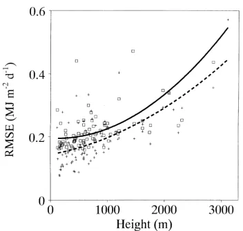
The quality of interpolation is demonstrated by the height–RMSE distribution of Fig. 1 and the spatial distribution of the RMSE values in Fig. 2. The rapid drop in quality of the interpolated data could be explained by the drop in station density with height and a possible increase of variability with height.
3.2. Approach 2: parameterisation of global radiation
Fig. 1. Solid curve and open squares: RMSE (Root Mean Square Error) vs height of first parameterised, then interpolated and cross validated global radiation. Dashed curve and crosses: RMSE of interpolated and cross validated observed global radiation. Daily data from 1994 to 1996.
The relationship between transmittance and cloudi-ness has been investigated by a number of authors (Kasten and Czeplak, 1980; Neuwirth, 1982). To illus-trate this relationship, a scatter plot of transmittance and cloud cover is shown from daily data at Innsbruck in Fig. 3. The maximum of the transmittance does not occur at 0 cloudiness, but at low cloudiness. This is not unique and not necessarily an artefact of the
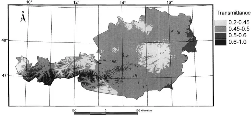
Fig. 2. Spatial distribution of the root mean square error from cross validating global radiation calculated from interpolated transmittances. Daily data from 1994 to 1996.
regression. Neuwirth (1982) compared mean values of the transmittance at different levels of cloudiness, corroborating the earlier mentioned observation.
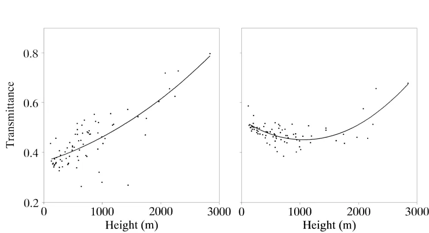
The transmittance–height relationship displays a pronounced seasonal cycle in Austria which is ob-viously governed by height, density and frequency of cloudiness (Fig. 4). High frequency of fog in low lying areas and of clear days at higher altitudes create a steep slope of the transmittance–height regression in Figs. 4 and 5. In spring, transmittance is still high at high altitudes, but the influence of foggy weather quickly disappears in Austria’s lowlands, and trans-mittance gains there a maximum in spring (Figs. 4 and 6). In May, the dullest places appear to be the medium altitudes at the northern and southern fringe of the Alps. Lifting of moist unstable air masses im-pinging on the Alpine chain promotes free convection, condensation, cloud cover and precipitation. During August spatial differentiation is at its minimum (not shown).
Fig. 3. The atmospheric transmittance–cloudiness relationship at Innsbruck. Transmittance was calculated from 3653 daily ratios of global/extraterrestrial radiation.
With the procedure described in Appendix A daily values of transmittance are calculated for each of Austria’s stations. Transmittance values are described as a function of cloudiness with a second degree polynomial:
¯ H ¯ H0
=a+bC+cC2 (1)
Fig. 4. Transmittance vs height for 105 stations in Austria for January (left) and May (right).
Cloudiness C calculated from three daily observations at 07:00, 14:00 and 19:00 hours local meantime with C=(C07+2C14+C19)/4 turned out to deliver much
better results than just a single daily observation.
¯
H0 represents a calculated reference radiation, for
instance, extraterrestrial radiation or direct radiation, andH¯ the measured global radiation. The coefficients
a, b, c from (1) were modelled as a function of station
elevation z as second independent variable:
a=a0+a1z+a2z2 (2)
b=b0+b1z+b2z2 (3)
c=c0+c1z+c2z2 (4)
individ-Fig. 5. Spatial distribution of long term mean values of atmospheric transmittance during January in Austria.
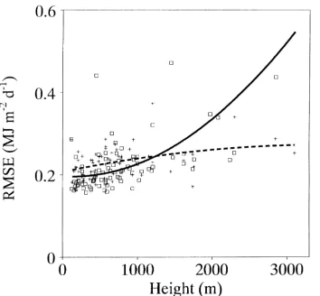
ual stations. It turned out that there is no significant difference between both validation results. One must conclude there is no significant horizontal variation in the regressed relationships. This is a major advantage compared with other parameterisation schemes using spatially highly variable atmospheric variables. The spatial distribution of the RMSE of the transmittances parameterised using Eqs. (1)–(4) and cross validated afterwards appears fairly homogeneous with only a slight deterioration at higher altitudes (Figs. 7 and 8 ).
Fig. 6. Spatial distribution of long term mean values of atmospheric transmittance during May in Austria.
Fig. 7. Solid curve and open squares: RMSE (Root Mean Square Error) vs height of first parameterised, then interpolated and cross validated global radiation. Dashed curve and crosses: RMSE vs height of parameterised and cross validated global radiation. Daily data from 1994 to 1996.
4. Comparison between Approach 1 and 2
It was expected that the density of cloud observing stations would be higher at higher elevations relative to global radiation observing stations. As a consequence the parameterisation approach should be able to com-pete with the interpolation of observed data (Fig. 9).
Fig. 8. Spatial distribution of the root mean square error, comparing time series of global radiation calculated from observed and parameterised atmospheric transmittances.
Fig. 9. Frequency distribution of cloud and global radiation ob-serving stations with altitude — total number of stations 303 and 105, respectively.
But differences in station density above 1500 m turned out to be insignificant.
elevation so that the power of explanation of the curves above 1000 m is strongly reduced. Interpolation of ob-served transmittances before 1992 produce unrealistic spatial distributions. For the time period previous to 1992 parameterisation could be more reliable for cer-tain areas with a low density of stations with global ra-diation observations. Data resources have not been ex-hausted for this project and adding observations from non-automatic stations could extend the application of interpolation as a method of choice to the time before 1992.
5. Conclusions
1. The parameterisation scheme for atmospheric transmittance appears spatially robust. There is practically no loss of quality through a generalisa-tion of the scheme for the whole region of Austria (84 000 km2), which includes complex terrain. 2. There is no significant loss of quality for lowlands
due to interpolation of parameterised atmospheric transmittance but a significant reduction of quality for areas above 1000 m.
3. The number of global radiation measuring sites has been increasing steadily during recent years so that interpolation has become a viable alternative to ac-quire radiation data either for a point or for an area of interest.
4. After 1992 interpolation is superior to parameteri-sation over most of Austria.
5. Areas at elevations above 1500 m still pose a prob-lem and require suppprob-lementary radiation informa-tion, for instance, provided by satellite data.
Acknowledgements
This study has been funded by the Austrian Fed-eral Ministry of Science and Transport and the FedFed-eral Ministry of Agriculture and Forestry. The research for this study was conducted when the first author was af-filiated with the Institute for Meteorology and Physics, University of Agriculture in Vienna. Philipp Weihs is thanked for his critical contributions.
Appendix A. The calculation of daily (monthly) average insolation on inclined surfaces
The approach used here for daily radiation sums follows a suggestion by Klein (1977) for daily aver-ages of a month. The daily radiationH¯Son an inclined
surface is
¯
HS=RH = ¯RK¯TH¯0 (A.1)
whereH¯ is the daily radiation sum on a horizontal
surface (MJ m−2/day);H¯0is the daily sum of the
ex-traterrestrial radiation (MJ m−2/day);R¯ is the ratio of the daily radiation on an inclined surface to that on a horizontal surface; and K¯T is the atmospheric
trans-mittance represented by the ratioH /¯ H¯0.
¯
R can be estimated for the direct and diffuse ra-diation and for the fraction which is reflected from the earth’s surface. Diffuse radiation is assumed to be isotropic and the earth’s albedo is kept constant for the area considered:
where H¯d is the daily sum of the diffuse radiation
(MJ m−2/day);R¯bis the ratio of the average direct or
extraterrestrial radiation on the inclined surface to that on a horizontal surface; s is the tilt of the surface from horizontal (degrees); andρis the surface albedo.
In order to apply this approach in complex terrain, atmospheric transmittance data have to be parame-terised or interpolated for the point or the area of in-terest.R¯
bwas set equal to the ratio of direct radiation
on the slope to direct radiation on a horizontal sur-face. Extraterrestrial radiation could also be used for this ratio.
When Eq. (A.2) is put into the second term of Eq. (A.1) three terms are created. The first term
¯
Hc=(H¯− ¯Hd)R¯b (A.3)
represents the direct radiationH¯c(global radiationH¯
minus diffuse radiation H¯d), which is modified by
slope, aspect and sky view of the receiving surface. This modification is taken into account by R¯b. The
¯ Hd
(1+coss)
2 (A.4)
describes the diffuse radiation taking into account the reduction of sky view by the slope. In case of a vertical wall, for instance, the cosine reduces to zero and only half the diffuse radiation is received from half of the hemisphere. The diffuse radiation is reduced not only by the slope but also by the surrounding terrain above the horizon, which results in the total reduction of the sky view expressed by h, the percentage of the sky hemisphere covered by terrain. Thus the expression (1+coss)/2 can be replaced by 1−h. The third term
¯
H ρ(1−coss)
2 (A.5)
describes the radiation, which is received from sur-faces projecting above the horizon. This term repre-sents in some sense the complement of Term 2 and therefore shows also the inverted sign. As mentioned earlier, the total sky view reduction h replaces the expression(1−coss)/2.
As measurements of H¯d are usually not available
on a routine base,H¯dis assessed from a few stations,
where diffuse radiation is measured. Neuwirth (1979) used the expression
to model the diffuse radiation.
In order to calculate the mean daily sums of the global radiation of a monthH¯S on an inclined surface
one can use the following expression:
¯
HS= ¯Rb(H¯ − ¯Hd)+ ¯Hd(1−h)+ ¯H ρh (A.7)
Therefore the mean daily sums of the global radiation on a horizontal surfaceH¯, the albedoρ, the total sky
view reduction h, the ratio of the direct or extraterres-trial radiation on an inclined to a horizontal surface
¯
Rband the diffuse radiationH¯dhave to be known.
Appendix B. The interpolation procedure
A height–transmittance relationship is deduced from daily atmospheric transmittance data of all avail-able stations. This relationship has been shown to be valid for the whole region:
Tj =a+bzj +cz2j+ · · · (B.1)
whereTjis the transmittance at station j; j has an index from 1 to n, the total number of available stations; a, b, c, . . . are the coefficients of the polynomial; and zj is the elevation (m) of station j.
In this work a second degree polynomial was applied. The coefficientsa, b, c, . . . were fitted by a generalisation of the least squares method for linear combinations of any functions (Press et al., 1992).
Based on the above fitted transmittance–height relationships, daily residualsRj at all n stations can be calculated:
Rj =(a+bzj +cz2j+ · · ·)−Tj (B.2)
In case Rj > 0(Rj < 0) transmittance at station j will be overestimated (underestimated) by Eq. (B.1). The field distribution of the residuals can be looked upon to be an approximation of the field which has its transmittance–height relationship removed.
The residuals of m selected neighbouring stations are multiplied by the weight of the inverse square of their distance to the point of interest. Therefore the inverse squared distances dij between the point of interest i and station j are summed up
Di =
The residual Ri at point i will be interpolated by weighing and summing the residualsRj of all selected m neighbouring stations
via the transmittance–height relationship and the in-terpolated residualRi at point i the transmittanceTi can be calculated:
Ti =Ri+(aj +bzj+cz2j+ · · ·) (B.5)
References
Bristow, K.L., Campbell, G.S., 1984. On the relationship between incoming solar radiation and daily maximum and minimum temperature. Agric. For. Meteorol. 31, 159–166.
Brühl, Chr., Zdunkowski, W., 1983. An approximate calculation method for parallel and diffuse solar irradiances on inclined surfaces in the presence of obstructing mountains or buildings. Arch. Meteorol. Geophys. Biocl., Ser. B 32, 111–129. Dirmhirn, I., 1951. Untersuchungen der Himmelsstrahlung
in den Ostalpen mit besonderer Berücksichtigung ihrer Höhenabhängigkeit. Arch. Meteorol. Geophys. Biokl., Ser. B. 2 (4), 301–346.
Duguay, C.R., 1993a. Radiation modelling in mountainous terrain: review and status. Mountain Res. Dev. 13, 339–357. Duguay, C.R., 1993b. Modelling the radiation budget of alpine
snowfields with remotely sensed data: model formulation and validation. Ann. Glaciol. 17, 288–294.
Duguay, C.R., 1995. An Approach to the estimation of surface net radiation in mountain areas using remote sensing and digital terrain data. Theor. Appl. Climatol. 52, 55–68.
Goldberg, B., Klein, W.H., McCartney, R.D., 1979. A comparison of some simple models used to predict solar irradiance on a horizontal surface. Solar Energy 23, 81–83.
Kasten, F., Czeplak, G., 1980. Solar and terrestrial radiation dependent on the amount and type of cloud. Solar Energy 24, 177–189.
Klein, S.A., 1977. Calculation of monthly average insolation on tilted surfaces. Solar Energy 19, 325–329.
Lexer, M., 1997. Simulation der Globalstrahlung aus täglichen Temperatur- und Niederschlagsdaten. Centralblatt für das gesamte Forstwesen 112 (2/3), 109–121.
Neuwirth, F., 1979. Beziehungen zwischen Globalstrahlung, Himmelsstrahlung und extraterrestrischer Strahlung in Österreich. Arch. Meteorol. Geophys. Biokl., Ser. B 27 1–13.
Neuwirth, F., 1982. Beziehungen zwischen den kurzwelligen Strahlungskomponenten auf die horizontale Fläche und der Bewölkung an ausgewählten Stationen in Österreich. Arch. Meteorol. Geophys. Biokl., Ser. B 30, 29–43.
Press, W.H., Teukolsky, S.A., Vetterling, W.T., Flannery, B.P., 1992. Numerical Recipes. Cambridge University Press, Cambridge, 963 pp.