Prediction of particle deposition on to rough surfaces
Andrew Michael Reynolds
∗Silsoe Research Institute, Wrest Park, Silsoe, Bedford MK45 4HS, UK Received 13 January 2000; received in revised form 5 April 2000; accepted 13 April 2000
Abstract
Lagrangian stochastic models applicable to the prediction of particle deposition onto hydraulically smooth surfaces are extended to account for the effects of surface roughness. Within the modelling approach, roughness elements are treated as mass ‘sinks’ volumetrically distributed within the flows. The extreme sensitivity of the deposition of micron and sub-micron sized particles to the micro-roughness of hydraulically smooth surfaces is shown to be very well predicted. This suggests that the models can be used to predict the deposition of particles onto leaves and other natural surfaces with micro-roughness elements correctly. Model predictions for the deposition velocities of spores and pollens onto completely rough sticky surfaces are shown to be in very close agreement with the experiment. © 2000 Elsevier Science B.V. All rights reserved.
Keywords:Deposition; Deposition velocity; Dispersal; Lagrangian simulation model; Spores; Pollens
1. Introduction
Despite there being considerable interest in the rates at which particles are transported from turbulent air flows to rough surfaces, relatively little progress has been made in the formulation of predictive models. Instead, attention has been focused largely upon parti-cle deposition to hydraulically smooth surfaces, i.e. to surfaces where the roughness elements do not protrude beyond the laminar sub-layer (see e.g. Hahn et al., 1985; Oron and Gutfinger, 1986; Fan and Ahmadi, 1993). A notable exception, however, is the work of Fernandez de la Mora and Friedlander (1982), and Schack et al. (1985) who developed a general corre-lation for particle deposition onto ‘completely’ rough surfaces, i.e. to surfaces having a roughness length
l+>70 (Schlictling, 1968) where, as throughout the manuscript, the superscript+is used to denote
quanti-∗Tel.:+44-1525-860000; fax:+44-1525-860156. E-mail address:[email protected] (A.M. Reynolds)
ties which have been rendered non-dimensional using the friction velocity,u∗, and the kinematic viscosity,ν. Although, the ability of this correlation to describe the available experimental data over nine orders of magni-tude of deposition velocity and covering three orders of magnitude in particle size, is impressive, the cor-relation contains two empirical factors which depend on the structure of the roughness layer and which can only be determined experimentally.
In this paper, a new, non-empirical, approach to predicting particle deposition onto rough surfaces is presented. The new approach is based upon the Lagrangian stochastic (LS) models of Reynolds (1999a,b) for the deposition of ‘heavy’ and ‘Brownian’ particles onto hydraulically smooth surfaces. The first model is applicable to the prediction of particle deposi-tion in the inertia-moderated and diffusion-impacdeposi-tion regimes. In these regimes, the deposition process is dominated by the effects of particle inertia and gradi-ent diffusion and so the effects of Brownian motion can be neglected. The second model is applicable
to the diffusion-deposition regime, where Brownian motion dominates the deposition process. It will be shown that these models are readily extendable to the prediction of particle deposition onto rough surfaces. The new modelling ingredients are the inclusion of a mass ‘sink’ volumetrically distributed within the flow field and the off-setting of the fluid velocity profile to account for the shift in the origin due to the presence of the roughness elements. The applicability of the models is thereby extended to include, for example, the deposition of spores and pollens onto grass and the capture of smaller particles by the micro-roughness elements on leaves and other natural surfaces. This ability will be demonstrated through detailed com-parisons with existing data from wind-tunnel and laboratory-scale experiments (Chamberlain, 1967; Wells and Chamberlain, 1967). In contrast with Eule-rian approaches to particle deposition (see e.g. Legg and Price, 1980; Slinn, 1982; Ferrandino and Aylor, 1985), the Lagrangian approach does not require the ad hoc specification of turbulent diffusivity and re-mains valid even when the length scale of the scalar field is much less than that of the turbulence. This oc-curs in the near-field of localized sources, in strongly inhomogeneous turbulence and in convective bound-ary layers. The Lagrangian approach has therefore the potential to find application in a diverse range of situations including the prediction of the dispersion and subsequent deposition, over complex terrain, of pollens from genetically modified crops and droplets from agricultural sprays, the prediction of acid depo-sition and predicting environmental aspects of safety in the nuclear and chemical industries.
2. Description of the LS model for heavy-particle deposition
The basis of the model is to regard the trajec-tories of ‘heavy’-particles in turbulent air flows as being like that of fluid-particles in a virtual fluid which has heavy-particle velocity statistics. That this, heavy-particle velocity statistics are regarded as be-ing, in some sense, perturbed fluid velocity statistics. Details of this approach to modelling the disper-sion and deposition of heavy-particles are given in Reynolds (1999a) and are described only briefly here. The heavy-particle velocity statistics, required here as model inputs, can be deduced from the fluid velocity
statistics and the equation of motion for a particle. The general equation of motion of a small, rigid particle in a turbulent flow contains many terms which can be jus-tifiably neglected in most incompressible air–particle systems when the particle density is much greater than the air density (Maxey and Riley, 1983). These neglected terms include the pressure gradient force, virtual mass, Basset history integral and Faxen’s mod-ification to Stokes’ drag force. For heavy-particles, Brownian motion can also be ignored. The equations of motion of the particle in a turbulent flow then reduce to a balance of Stokes’ drags force, particle inertia and any body forces which may be present
duuup
whereupis the particle velocity,uf is the local fluid velocity, aB is the acceleration due to body forces and τp is the particle aerodynamic response time,
which according to Stokes’ drag law is given by
τp=(ρp/ρf)dp2/18ν whereρpis the particle density, ρf is the fluid density, dp is the particle diameter
andν is the kinematic viscosity. The dominant body forces acting on a heavy-particle are lifted due to mean shear (Saffman lift) and turbophoresis which is a convective drift down gradients of velocity variance and gravity. These are described by
FL =1.62
where duf/dyis the gradient in the local mean stream-wise air velocity,vpandvfare the components of fluid
velocity and particle velocity in the direction normal to the streamwise direction, respectively, σp is the
root-mean-square (rms) value ofvpandg=9.81 m s−2
is the acceleration due to gravity. Other forces such as lift caused by free rotation can be shown to be at least an order of magnitude less than the shear lift and so they can be ignored (Kallio and Reeks, 1989). Provided that the fractional changes in 1σp/σp
during time increments of size,τp, are much less than
unity, Eq. (1) implies that the mean value of normal particle velocitiesvp=τpaB, and that the rms normal
particle velocities are related to the rms normal fluid velocities byσp2=σf2/(1+τp/T′
timescale associated with fluid velocity fluctuations along a particle trajectory. This timescale is shorter than the Lagrangian timescale,TL, for fluid-particles
along a fluid-particle trajectory. This is simply because of the effects of particle-inertia and gravity which cause the trajectory of a heavy-particle to deviate from that of the fluid-particle containing it at any instant, with the consequence that fluid-velocity correlations along a heavy-particle trajectory decay more rapidly than those along a fluid-particle trajectory (Csanady, 1963). Here, following Sawford and Guest (1991), this ‘crossing-trajectories effect’ is parameterized by
TL′ =TL(1+(βvp/σf)2)−(1/2), whereβis an
empiri-cal constant of O(1) relating Lagrangian and Eulerian turbulence scales. Sawford and Guest (1991) deter-mined the value of β by optimizing the agreement between the predicted and measured dispersion of tracers in decaying grid turbulence. They estimated that β=1.5, which is the value adopted here. Other values of β∼O(1) were not found to lead to signif-icantly different predictions for particle deposition. The Lagrangian timescale TL = 2σf2/C0ε, where ε
is the mean rate of dissipation of turbulent kinetic energy divided by fluid density and C0 is the La-grangian velocity structure function constant. Here we takeC=5 (Reynolds, 1998a).
It is not necessary to consider third- and higher-moments of the heavy-particle velocity statistics, as these are of secondary importance in determin-ing the trajectories of heavy-particles in turbulent shear-layers. More important are the effects of the strong gradients in Reynolds-stress (Reynolds, 1999a). Consequently it is sufficient to regard the heavy-particle velocities as being Gaussian. Further-more, because root-mean square turbulent velocity fluctuations in the streamwise direction are typically small compared to the mean streamwise velocity, it is sufficient to consider only turbulent particle motions in the direction normal to the surface.
The one-dimensional LS model which satisfies the well-mixed condition (Thomson, 1987) for Gaussian heavy-particle velocity statistics is given by
dxp
ing particle velocities along the particle trajectory, dξ
are increments of an independent Wiener process with mean of zero and variance of dt, and where
ap =
The generalization of Eqs. (3) and (4) to two and three dimensions gives rise to the so-called ‘non-uniqueness problem’, familiar in the context of LS models for tracer-particles. This non-uniqueness is non-trivial because different LS models produce different predictions for mean particle concentra-tions (Sawford and Guest, 1988). Criteria in addition to the well-mixed condition which can resolve this non-uniqueness have yet to be established (Reynolds, 1998b,c; Sawford, 1999).
Particle trajectories were simulated by numerical integration of Eqs. (3) and (4). Following Thomson (1987) the size of the time-step, used in this integra-tion, is taken to be
dt =min
which ensures that the simulated trajectories resolve any inhomogenities in σp and TLp. In the numerical simulations, particles were perfectly reflected when they reached the top of the boundary-layer. This does not result in any violation of the well-mixed condition when the particle velocity statistics are taken to be Gaussian (Wilson and Flesch, 1993) and is equivalent to the imposition of a no-net-flux boundary-condition.
3. Lagrangian stochastic model for Brownian particle deposition
turbu-lent dispersion and Brownian motion. The basis of the model is to partition turbulent and Brownian motions. This is justifiable because the timescales governing Brownian motion are much smaller than the smallest timescale, the Lagrangian dissipation timescale, td, associated with turbulent motions.
De-tails of this model can be found in Reynolds (1999b). The model, which satisfies the well-mixed condition for the joint turbulent–Brownian process, is given by
dxp
where dξ and dξ′ are components of independent Wiener processes with means of zero and variances of dt,D=kTτp/mpis the Brownian diffusion constant,
kis the Boltzman constant,Tis absolute temperature andmp is the particle mass. Turbulent and Brownian particle motions in the streamwise direction are taken to be negligible compared to advection by the mean air flow. The Lagrangian timescale is taken to be
TL=2σv2/C0′ε, where the difference betweenC0′ and
C0 accounts for Reynolds number effects, which are
of importance in determining the trajectories of Brow-nian particles close to surfaces. The two constants,
C0′ andC0, are related by C0′ =C0′/(1+Re∗−(1/2)) where Re∗ is the Lagrangian Reynolds number (Sawford, 1991). The Lagrangian Reynolds number Re∗=(TL/td)2, wheretd=C0/2a0tη,tη is the Eulerian
dissipative timescale, a0 = 0.13Re0λ.64 is a constant
related to the rms of fluid-particle accelerations and Reλ is the Reynolds number based on the Taylor
micro-scale. Here, because different fluid-particle tra-jectories contribute to the trajectory of a Brownian particle, C0 is not the Lagrangian velocity structure
function constant. The value ofC0, the only adjustable
model parameter, was determined by optimizing model agreement with the experiment deposition data of Wells and Chamberlain (1967). This gaveC0=5.
The trajectories of micron and sub-micron sized particles were simulated by numerical integration of Eq. (6) using a time-step analogous to that given in Eq. (5) for heavy-particles. By following the approach adopted in Section 2, the model could be readily ex-tended to include the effects of gravity but this is not necessary here since model predictions will later be compared with experimental data for deposition from vertical pipe flow. Gravity is known (see e.g. Young and Leeming, 1997) to have a negligible effect upon deposition from the vertical flows. The generalization of the model to two and three dimensions of problem-atic because of the non-uniqueness problem.
4. Mass sink and velocity off-set
The predominant effect of surface roughness is to shift the virtual origin of the velocity profile by a dis-tance,e=0.55l, away from the surface, wherelis the length of the protrusions (Wood, 1981). Now, because much of the area available for particle deposition is at the protrusions themselves rather than the bottom sur-face of the boundary-layer and because the turbulent motion of particles is more intense around the protru-sions than at the bottom surface, a large fraction of particle deposition is expected to occur at the effec-tive roughness height. In the modelling approach, it is therefore assumed that particles are captured when they reach the level of the effective roughness height
b=l−e=0.45l above the origin, e, of the velocity profile.
The capture efficiency is taken to be unity and once captured particles are assumed not to rebound or to subsequently become detached. This is appropriate to situations where the deposition surface has been made ‘sticky’, as is the case in some of the wind-tunnel studies of deposition by Chamberlain (1967), against which models will be validated. It is also applicable to the micron and sub-micron sized particles which on making contact with a surface are likely to be deposited and remain deposited.
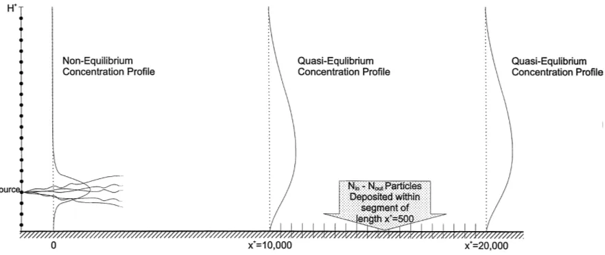
Fig. 1. Schematic representation of the procedure used to calculate deposition velocities from the particle trajectories simulated by the LS models.
simply ignoring any contributions to rebound from streamwise velocity fluctuations and retaining a one-dimensional LS model but without a rigorous means for determining capture efficiencies and bounce back velocities the resulting model will be ad hoc in character.
5. Prediction of deposition velocities
In the simulations, as in the experiments of Wells and Chamberlain (1967), and Chamberlain (1967), the velocity of deposition,Vdep, is taken to be the ratio of
the flux of particles to the mass sink,j, divided by the mean concentration of particles,hci. The prescription for the calculation of this flux from the particle trajec-tories simulated by the LS models is described below and illustrated schematically in Fig. 1.
The one-dimensional form of the particle deposi-tion flux through an incremental length1X is given byj=(dN/dt)/1XwhereN=hci1XHis the number of particles within a ‘volume’1XHof a boundary-layer of heightH. Therefore, dN/dt=−VdepN/Hwhich upon integration yields N(t)=N(0) exp(−Vdept/H). This
expression could be used to calculate deposition ve-locities once the numbers of airborne particles,N(0) andN(t), within the sample volume at times 0 and t
have been predicted from the trajectories of particles
simulated using the LS models described in Sections 2 and 3. However, it is more natural to calculate de-position velocities from the number of airborne parti-cles,NinandNout, flowing into and out of the sample
volume. This is readily achieved by expressing timet
in terms of the average streamwise velocity across the boundary-layer,U, and the lengthX. SubstitutingX/U
fortinto the expression forN(t) and rearranging gives
Vdep=HU/Xln(Nin/Nout), which is the expression used
here to calculate the deposition velocity, Vdep. It is
identical to that utilized by Swailes and Reeks (1994) in their numerical simulations of particle deposition from turbulent duct flows and is directly analogous to
Vdep=RU/2Xln(Nin/Nout) which has been much used in the prediction of particle deposition in pipes of radius R (Kallio and Reeks, 1989; Uijttewaal and Oliemans, 1996).
particle concentration profile and deposition as a function of streamwise location until steady values were attained. That is, the equilibrium deposition rate was determined from the deposition velocities calculated for 20 segments of length X+=500 of a sample volume of the boundary-layer located between
X+=10,000 andX+=20,000 downwind of the source. To promote the establishment of the quasi-equilibrium concentration particles were released from 20 equis-paced positions between the deposition surface and the top of the boundary-layer. It was further promoted by releasing particles with velocities drawn from the local equilibrium Gaussian velocity distributions. It is assumed that the introduction of particles into the boundary-layer does not affect the statistical proper-ties of the airflow required here as model inputs.
6. Comparisons of predicted and measured deposition velocities
6.1. Wind tunnel experiments of Chamberlain (1967)
Chamberlain (1967) measured the deposition veloc-ities of spores and smaller particles in a wind-tunnel neutral boundary-layer to a variety of surfaces which were, depending on the value ofu∗, either ‘completely’ rough or in the transition regime between being hy-draulically smooth and completely rough. The geom-etry of Chamberlain’s experiment is similar to that shown in Fig. 1. The particles were tagged with a radioactive marker and the numbers of particles de-posited was measured from the radioactivity on the deposition surfaces. The radioactivity of the particles in the airstream was determined from the average ra-dioactivity of particles caught in a sampler. The de-position surfaces included Italian rye grass grown to a height of 60 mm, artificial grass made of strips of PVC of length 80 mm and treated with a sticky so-lution, and rough glass with pyramidal roughness el-ements about 3 mm high, made sticky with stopcock grease. The corresponding values of roughness length
z0are 10, 0.65 and 0.2 mm.
The ‘sticky’ surfaces are of particular interest be-cause the number of particles striking these surfaces, a quantity which can be predicted directly by the LS models, can be equated with the number of particles being deposited.
In the experiments of Chamberlain, the source ef-fectively extended across the boundary-layer, which here is taken to be homogeneous in the cross-wind direction. It is, therefore, appropriate in the nu-merical simulations of these experiments to ne-glect particle motions in the cross-wind direction and use a one-dimensional LS model for particle motions in the vertical direction along with the one-dimensional calculation of deposition velocities described in Section 5. The LS models require the mean streamwise velocity,uf, and root-mean-square fluctuating velocity, σv and the mean dissipation rate of turbulent kinetic energy as model inputs. The boundary-layer had a logarithmic mean velocity profile. Therefore,
Kármán constant. Chamberlain (1967) did not report upon profiles of rms normal velocities. However, for the larger particles considered by Chamberlain (1967), the Lycopodium spores and ragweed pollen, which have mean diameters of 32 and 19mm and density ρ=1175 kg m−3, gradient-diffusion plays little or no
part in determining deposition as these particles, by acquiring sufficient momentum from the large turbu-lent eddies in the turbuturbu-lent core of the flow, reach the deposition surfaces directly. That is, for all the values ofu∗appropriate to the experiments of Chamberlain (1967), the Lycopodium spores and ragweed pollen have non-dimensional relaxation timescalesτp+>20, which corresponds to the ‘inertia-moderated regime’ of particle deposition. Consequently for these particles it is appropriate to treat the rms normal fluid velocity as a constant throughout the boundary-layer. Following Pasquill (1974), this constant is taken to beσf=1.3u∗. It should be noted, however, that even whenσfis
con-stant, there is a weak turbophoretic force because of the dependency ofσponTLp(yp).
Fig. 2. Comparison of predicted (s) and measured (d; Chamberlain, 1967) deposition velocities,Vdep, as a function of friction velocity,
u∗, forLycopodiumspores from a wind-tunnel neutral boundary-layer to sticky artificial grass.
Fig. 3. Comparison of predicted (s) and measured (d; Chamberlain, 1967) deposition velocities,Vdep, as a function of friction velocity,
Fig. 4. Comparison of predicted (s) and measured (d; Chamberlain, 1967) deposition velocities,Vdep, as a function of friction velocity,
u∗, forLycopodiumspores from a wind-tunnel neutral boundary-layer to sticky rough glass.
velocity, u∗, the length of the protrusions, l, and particle size,dp.
The good agreement between the model and exper-imental measurements of deposition is already under-stood. The wind spread at the height of the tips of the artificial grass is equal to approximately 2u∗ and if u∗ is say 0.5 m s−1 then the stopping distance of
Lycopodium spores travelling at this speed is 3 mm which is comparable with the width, 5 mm, of the ar-tificial grass. The efficiency of collection of the tips of the grass will therefore be quite high at high wind speeds. At low wind speeds the efficiency will be small, but the corresponding reduction in deposition by impaction is masked because sedimentation then becomes relatively more important. The same remarks also apply to deposition on to rough glass because in this case the roughness length (3 mm) is less than the stopping distance of theLycopodiumspores when
u∗≥0.2 m s−1.
Slinn (1982) obtained comparable agreement with the deposition data of Chamberlain (1967) using an Eulerian approach with a turbulent-eddy diffusivity closure; an approach which was later refined by Fer-randino and Aylor (1984). However, as noted earlier, such closures are essentially ad hoc in character and
their validity is severely restricted. A further difficulty is that, unlike in the Lagrangian approach where depo-sition velocities are calculated directly, in Eulerian ap-proaches deposition velocities are inferred indirectly from predicted particle fluxes.
Chamberlain’s (1967) experimental data for depo-sition to real grass shown in Fig. 5 are in marked con-trast with those for artificial grass, with the values of
bound-Fig. 5. Comparison of predicted (s) and measured (d; Chamberlain, 1967) deposition velocities,Vdep, as a function of friction velocity,
u∗, forLycopodiumspores from a wind-tunnel neutral boundary-layer to real grass.
ary layer of the air flow. Given capture efficiencies less than unity and the importance of rebound in deter-mining the transport ofLycopodiumspores, it is there-fore not surprising that the model is seen in Fig. 5 to over-predict deposition to real grass.
The deposition velocities of the smaller particles (particles of polystyrene with mean diameter 5mm,
droplets of tricresylphosphate with mean diameters of 2 and 1mm, and Aitken nuclei with mean diameter
0.08mm) onto artificial grass were under-predicted by
two or more orders of magnitude, with Brownian mo-tions predicted to make an insignificant contribution to particle deposition. For these particles, unlike for the spores, gradient-diffusion (turbophoresis) is an impor-tant transport mechanism. Indeed, it dominates particle transport in the ‘diffusion’ and ‘diffusion-impaction’ regimes (Young and Leeming, 1997). Gradient diffu-sion is unlikely to be well described with the adopted parameterization of normal rms fluid velocities. Un-fortunately without experimental data, it is difficult to improve upon this parameterization. In the next sec-tion, it will be shown that when normal rms fluid ve-locities are known, the deposition veve-locities of micron and sub-micron size particles can be accurately pre-dicted.
6.2. Experiments of Wells and Chamberlain (1967)
Wells and Chamberlain (1967) measured the deposition velocities of Aitken nuclei, droplets of tricresylphosphate and particles of polystyrene onto a cylindrical rod placed axially within a vertical fully-developed turbulent pipe flow. For the ex-periments of Wells and Chamberlain (1967), the non-dimensional aerodynamic response times of these particles lie predominantly within the ‘diffusion-deposition’ regime and so Brownian motions domi-nated the deposition process. Both the cylinder and the pipe were earthed to avoid electrostatic effects. Wells and Chamberlain (1967) considered two depo-sition surfaces: brass which was hydraulically smooth and filter paper which had fibres of mean length 100mm (l+<10) and was, depending on the value
of u∗, either hydraulically smooth or close to being hydraulically smooth.
Deposition velocities are principally determined by the characteristics of the near-wall turbulent boundary, which are largely insensitive to geometric detail pro-vided of course that there are no recirculation zones and stream-line curvature is negligible. This has been strikingly illustrated by Young and Leeming (1997) who showed that measurements of deposition veloci-ties from a diverse range of experiments collapse onto a narrow band of values when quantities are appro-priately non-dimensionalized using the friction veloc-ity and the kinematic viscosveloc-ity. It is therefore legiti-mate to compare the experimental data of Wells and Chamberlain (1967) with predictions obtained from LS models for particle deposition from fully devel-oped turbulent pipe flow onto the pipe itself. This is advantageous because unlike for the flow utilized by Wells and Chamberlain (1967), the flow characteristics of fully-developed turbulent pipe flow are accurately known. Moreover, the axial symmetry of the pipe fa-cilities of the use of one-dimensional LS model along with the one-dimensional treatment of deposition are described in Section 5.
Model predictions were obtained using the LS model for Brownian particles, assuming that the deposition surfaces were located at 0mm and
0.45mm×100mm. This LS model is strictly
appropri-ate only for non-dimensional aerodynamic response times, 0.1<τp+, because then deposition is dominated by Brownian diffusion within a very thin layer di-rectly adjacent to the deposition surface. For larger values of σp+, the effects of particle inertia, which are not account for in the model, become important in determining particle deposition. The fluid velocity statistics required for these simulations are taken from Reynolds (1999b) and references therein
uf+=y+ y+≤5
u+f = −0.076+1.445y+−0.0488y+2+0.0005813y+3 5< y+<30
uf+=2.5 lny++5.5 y+≥30
σv+=
0.005y+2
1+0.002923y+2.128 ε+= 2.5
y+ y+>30
ε+= 2.5
30 y
+<+30
(8)
The form of the mean velocity in the buffer zone (5<y+<30), obtained by Kallio and Reeks (1989)
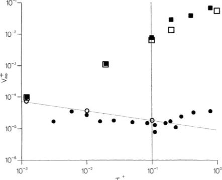
Fig. 6. Comparison of predicted (open symbols and the dotted line) and measured (solid symbols: Wells and Chamberlain, 1967) de-position velocities,Vdep+, of Brownian particles with aerodynamic response times,τ+. Deposition velocities are shown for two dif-ferent hydraulically smooth surfaces; smooth brass (circles) and filter paper having 100mm fibres (squares). The model is strictly
applicable only in the ‘diffusion regime’. The boundary between the diffusion and diffusion-impaction regimes is indicated by the vertical dotted-line. The superscript+refers to quantities which have been rendered non-dimensional using the friction velocity, u∗, and the kinematic viscosity,ν.
using cubic spline interpolation, ensures that the velocity gradient is continuous throughout the boundary-layer. The forms for the velocity variance and mean dissipation rate fits to experimental data and data from direct numerical simulations.
aerodynamic response time,τp=(ρp/ρf)dp2/18ν(1+
2.7Kn), where Kn=λ/dp is the particle Knudsen
number. The ‘correction factor’ (1+2.7Kn), due to Cunningham (1910), accounts for the deviations from Stoke’s drag law which occur when the parti-cle diameter is comparable with the molecular mean free path, λ. When presented as a function of τp+
and in the absence of surface roughness elements, it is easily shown that deposition velocities in the ‘diffusion-deposition’ regime depend on the similarity parameter (τ+
p /Sc2)1/3, where Sc=ν/Dpis the Schmit
number (Young and Leeming, 1997). This parameter is independent of particle size if rarefied gas effects. In close agreement with experiment, the model predicts that Vdep+=0.06Sc−(2/3)
=0.06(τp+/Sc2)1/3τ+ p−(1/3).
Fig. 6 also shows that the model correctly predicts the considerable enhancement in deposition when the deposition surface is covered with a filter paper hav-ing fibres too small to disturb the laminar sub-layer. In contrast with other modelling approaches for rough surfaces (e.g. Wood, 1980; Fan and Ahmadi, 1993) but in agreement with the experimental data of Wells and Chamberlain (1967), predicted deposition velocities are seen not to become almost indepen-dent of particle aerodynamic response times in the ‘diffusion-deposition’ regime, at least for the rough-ness under consideration.
7. Conclusions
Lagrangian stochastic models for the dispersion and deposition of ‘heavy’ and ‘Brownian’ particles have been extended to account for surface roughness. The approach offers a simple, fast and reliable com-putational tool of practical use which is applicable to surfaces, ranging from hydraulically smooth to completely rough. Model predictions compared very favourably with the measured deposition velocities of spores to artificial sticky grass and sticky rough glass and with the deposition of micron and sub-micron sized particles to hydraulically smooth surfaces. The success of the model for Brownian-particle deposi-tion suggests that the model can predict correctly the deposition of sub-micron sized particles onto leaves and other natural surfaces with micro-roughness ele-ments. Deposition velocities of spores onto real grass were, however, over predicted. It was suggested that
this was because the capture efficiency of real grass is significantly different from unity, which results in significant differences between the numbers of particles which strike the grass, which in the model are assumed to deposit, and the numbers of particles which actually deposit. Extending the model to sur-faces having capture efficiencies less than unity is problematic because rebound is determined in part by the streamwise velocity variance of the air flow and incorporating this quantity into LS models leads to a non-uniqueness problem. This difficulty could be circumvented by simply ignoring any contributions to rebound from streamwise velocity fluctuations and retaining a one-dimensional LS model but without a rigorous means for determining capture efficiencies and bounce back velocities the resulting model will be ad hoc in character.
References
Chamberlain, A.C., 1967. Transport of Lycopodiumspores and other small particles to rough surfaces. Proc. R. Soc. 296A, 45–70.
Csanady, G.T., 1963. Turbulent diffusion of heavy particles in the atmosphere. J. Atmos. Sci. 20, 201–208.
Cunningham, E., 1910. On the velocity of steady fall of spherical particles through fluid medium. Proc. R. Soc. London, Ser. A 83, 357–365.
Fan, F.-G., Ahmadi, G., 1993. A sublayer model for turbulent deposition of particles in vertical ducts with smooth and rough surfaces. J. Aerosol. Sci. 24, 45–64.
Fernandez de la Mora, F., Friedlander, S.K., 1982. Aerosol and gas deposition to fully rough surfaces: filtration model for blade-shaped elements. Int. J. Heat Mass Transfer 26, 1725– 1735.
Ferrandino, F.J., Aylor, D.E., 1985. An explicit equation for deposition velocity. Boundary-Layer Meteorol. 31, 197–201.
Hahn, L.A., Stukel, J.J., Leong, K.H., Hopke, P.K., 1985. Turbulent deposition of submicron particles on rough walls. J. Aerosol. Sci. 16, 81–86.
Kallio, G.A., Reeks, M.W., 1989. A numerical simulation of particle deposition in turbulent boundary layers. Int. J. Multiphase Flow 15, 433–446.
Legg, B.J., Price, R.I., 1980. The contribution of sedimentation to aerosol deposition to vegetation with a large leaf area index. Atmos. Environ. 14, 305–309.
Maxey, M.R., Riley, J.J., 1983. Equation of motion for a small rigid sphere in a nonuniform flow. Phys. Fluids 26, 883–889.
Oron, A., Gutfinger, C., 1986. On turbulent deposition of particles to rough surfaces. J. Aerosol. Sci. 17, 903–920.
Reynolds, A.M., 1998a. Comments on the universality of the Lagrangian velocity structure function constant (C0) across
different kinds of turbulence. Boundary-Layer Meteorol. 89, 161–170.
Reynolds, A.M., 1998b. On the formulation of Lagrangian stochastic models of scalar dispersion within plant canopies. Boundary-Layer Meteorol. 86, 333–344.
Reynolds, A.M., 1998c. On trajectory curvature as a selection criterion for valid Lagrangian stochastic dispersion models. Boundary-Layer Meteorol. 88, 77–86.
Reynolds, A.M., 1999a. A Lagrangian stochastic model for heavy particle deposition. J. Colloid Interface Sci. 215, 85–91. Reynolds, A.M., 1999b. A Lagrangian stochastic model for the
dispersion and deposition of Brownian particles. J. Colloid Interface Sci. 217, 348–356.
Sawford, B.L., 1991. Reynolds number effects in Lagrangian stochastic models of turbulent dispersion. Phys. Fluids A3, 1577–1686.
Sawford, B.L., 1999. Rotation of trajectories in Lagrangian stochastic models of turbulent dispersion. Boundary-Layer Meteorol. 93, 411–424.
Sawford, B.L., Guest, F.M., 1988. Uniqueness and universality of Lagrangian stochastic models of turbulent dispersion. In: Proceedings of the 8th Symposium on Turbulence and Diffusion, American Meteorology Society, Boston, USA, pp. 96–99.
Schack Jr., C.J., Pratsinis, S.E., Friedlander, S.K., 1985. A general correlation for deposition of suspended particles from turbulent gases to completely rough surfaces. Atmos. Environ. 19, 953–960.
Schlictling, H., 1968. Boundary Layer Theory. Springer, Berlin. Slinn, W.G.N., 1982. Predictions for particle deposition to
vegetative canopies. Atmos. Environ. 16, 1785–1794. Swailes, D.C., Reeks, M.W., 1994. Particle deposition from a
turbulent flow. I. A steady-state model for high inertia particles. Phys. Fluids 6, 3392–3403.
Thomson, D.J., 1987. Criteria for the selection of stochastic models of particle trajectories in turbulent flows. J. Fluid Mech. 180, 529–556.
Uijttewaal, W.S.J., Oliemans, R.V.A., 1996. Particle dispersion and deposition in direct numerical and large eddy simulations of vertical pipe flows. Phys. Fluids 8, 2590–2604.
Wells, A.C., Chamberlain, A.C., 1967. Transport of small particles to vertical surfaces. Br. J. Appl. Phys. 18, 1793–1799. Wilson, J.D., Flesch, T.K., 1993. Flow boundaries in random-flight
dispersion models: enforcing the well-mixed condition. J. Appl. Meteorol. 32, 1695–1707.
Wood, N.B., 1981. A simple method for the calculation of turbulent deposition to smooth and rough surfaces. J. Aerosol. Sci. 12, 275–290.