COMPUTING THE AUTOPILOT CONTROL ALGORITHM USING
PREDICTIVE FUNCTIONAL CONTROL FOR UNSTABLE MODEL
H. A. KASDIRIN
DR
J.
A. ROSSITER
(2009 International Conference of Soft Computing and Pattern Recognition)
UNIVERSITI TEKNIKAL MALAYSIA MELAKA
2009 International Conference of Soft Computing and Pattern Recognition
Computing The Autopilot Control Algorithm using Predictive Functional
Control for Unstable Model
H. A. Kasdirin,
Faculty of Electrical Engineering, Universiti Teknikal Malaysia Melaka, Malaysia
Phone: +606-555 2215, Fax: +606-555 2222, Email: [email protected]
Abstract-This paper discusses the computing development of a control algorithm using Predictive Functional Control (PFC) for model-based that having one or more unstable poles. One basic Ballistic Missile model (10) is used as an unstable model to formulate the control law algorithm using PFC. PFC algorithm development is computationally simple as a controller and it is not very complicated as the function of a
missile will explode as it reaches the target.
Furthermore, the analysis and issues of the
implementation relating linear discrete-time unstable process are also being discussed. Hence, designed PFC algorithm need to find the suitable tuning parameters as its play an important part of the designing the autopilot controller. Thus, the tuning of the desired time constant, 'I' and small coincidence horizon n1 in a single
coincidence point shows that the PFC control law is built better in the dynamic pole of the unstable missile mode. As a result, by using a trajectory set-point, some positive results is presented and discussed as the missile follow its reference trajectory via some simulation using MATLAB 7.0.
Keywords: Predictive Functional Control (PFC), autopilot design, state-space models
I. INTRODUCTION/BACKGROUND
Predictive Functional Control (PFC), which developed by Richalet [l] is one of Model Predictive Control (MPC) techniques that have been developed as a powerful algorithm for controlling process plants [6]. PFC is based on the same approach with all MPC strategies i.e., prediction of the future outputs, and calculation of the manipulated variables for an optimal control [4]. Therefore, PFC is also based on the same principles which are using an internal model,
specification of a reference trajectory and
determination of the control law. In this paper, the focus is on the computing implementation of the PFC algorithm on an unstable model-based automation application that is in fast response such as the missile dynamic models.
Based on the aim and objectives given above, this project is computing the control algorithm design an autopilot system of a guided missile using PFC controller. Thus, this paper will be started with the
computation development theory of the PFC
algorithm. The second section will be looked the problem formulation by introducing an unstable
Dr J. A. Rossiter
Department of Automatic Control & Systems
Engineering
The University of Sheffield, UK Email: [email protected]
model and the formulation of its control law. This section also will be discussing the way PFC handle the unstable process by pre-stabilise the unstable plants to implement the stabilizing linear PFC control formulation.
The last section will then jumped into the simulation and implementation result of PFC on the model-based. The section will be explained how PFC algorithm could work in given unstable model and then further the implementation of PFC whether PFC could work as a controller on fast process by given a specific set-point. The last section of this project tries to conclude the project as it developed from previous section. The summary of the project will be discussed and some recommendations will be noted for further analysis and research.
11. PREDICTIVE FUNCTIONAL CONTROL
This section will be discussing the theoretical part of control law so that it can be formulated and implemented in the following sections. However, at first, this section will describe the introduction of PFC algorithm and continued with the formulation of its control law.
A. Formation of Model-based controller
The model is the essential element of an MPC controller and hence, also for PFC controller. PFC can use many forms of model i.e.; internal model (IM), including state space, transfer function, Finite Impulse Response (FIR), fuzzy rules, and etc [5],[6]. The use of IM is important in PFC to capture the process dynamics of the system and also continue to calculate the PFC control law later on.
Hence, for this section, the model is developed in
state-space form. The discussion
of
PFC and otherMPC algorithms in state-space form has several
advantages, including easy generalisation to
multivariable systems, ease of analysis of closed-loop properties, and online computation [6].
Given the general state space model, of the form:
セォKエ@
=
aセォ@+
By_k
セォ@
=
cセォ@+
Dy_k
(2.1)
Prediction with a strictly proper system (D = [O]), so
:!k+2
=
A:!k+i+
B!ik+iY
=Cx
-k+2 -k+2
(2.2)
From Equation 2.1 and 2.2 above, it shows the model used is a linear one that could represent by;
セォ@
=Pxx:!k +Hxl:!.k-1セォ@
=
P,!k+
Hl:!.k-1(2.3)
where&< is the state model, 1!i< is the input model,» is
the measured output model, Pxx• Hxx , P and H are
respectively, matrices or vectors of the right dimension by using the state-space approach.
The advantages of developing the PFC algorithm are that by its intuitive approach. However, before deriving the PFC control law, there are some criteria needed to look at which are the formulation its reference trajectory, the coincidence points (if occurs) as well as its future control trajectory. Hence, assuming at a single coincidence point and Y. k - ; = Y.
k· the PFC control law can be computed by rewriting
the Equation 2.3 and obtained;
y_ k = - HJ [ P ,! k + ( rk - (rk - y,J 'P; ) ]
Y.k = -K,!k + /Jrk (2.4)
where; K = - H1 ( P- 'P' Yk)
fJ
= -HJ (I - 'P;)Thus, it can easily express as a fixed linear feedback law in the form of prediction algorithm. Hence, the conventional a posterior stability and sensitivity analysis can be applied in straightforward manner.
B. Unstable Model Using PFC Algorithm
PFC algorithm is defined in the previous sub-section is basically open-loop process control applications. In the contrary, in industry applications, open-loop unstable processes do also occur. Yet, these systems are difficult to control. Therefore, systematic control design tools are needed to handle complex instability without a high on-line computational load. ADERSA have successfully applied PFC on many unstable systems [3]. This section will discuss the theoretical tools to pre-stabilise the unstable plants to
implement the stabilizing linear PFC control
formulation.
PFC, as well as other MPC algorithms are weak with both non-minimum phase problems and some unstable process [3], or called prediction mismatch. If the process open-loop is unstable, PFC is ill-posed because prediction cannot match desired behaviour of the process, i.e. diverging. Therefore, divergence
168
open-loop prediction is the main cause of the prediction mismatch. Hence, there is a must to stabilise the prediction. There are two ways of pre-stabilise the predictions which are inserting a stabilising loop and another by shaping the future inputs, algebraically so that the outputs are stable. However, this section only focused on solving algebraically the unstable process as discussed by [7] and [8].
C. Predictive Stabilisation
Removal of the prediction mismatch is essential for PFC to work. Hence, the model needs to have prediction stabilisation. One method is by cancelling the unstable modes and starts working with stable predictions [8]. This means that the PFC control law must be modified. Therefore, in solving this problems PFC will lead to good closed-loop performance if the predictions used are a good match to the consequent closed-loop behaviour.
The illustration below shows the state space method of predictions to cancel the unstable modes [3]. From Equation 2.1, let the state-space matrix have some unstable eigenvalues. Decompose the system into stable and unstable modes using eigenvalue decomposition;
A = [ W,, Wu ] diag [ /1.1,
-TJ
Au] V,_y/
(2.5)where; subscript s is used for stable and u for
unstable.
The control law becomes,
!:!.k- I = - [ W,A/ V,7
r
1 V/A' :!k + H(J.H. k = - K :! k + H/J (2.6)
where K = [ W, /1/ V/
r
1 V/ A1 andfJ
could bechoose freely.
Consequently, the main concepts of PFC and its algorithm have been discussed. This section is really important before introducing an example of fast
system which is missile models and the
implementation of the algorithm, elaborated in this section.
III. PROBLEM FORMULATION OF THE AUTOMATION FAST-RESPONSE MODEL
vector and become a free-falling body after engine cut-off [IO].
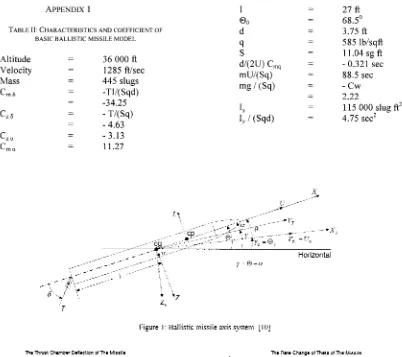
The main feature of the missile as shown in Figure 1 is that it is roll-stabilised; thus there is no coupling between longitudinal and lateral mode which simplifies the analysis. Another feature is that its trajectory is planned to maintain the missile at a zero angle of attack. Based on the assumption made above, the Ballistic Missile Model can be represented by its dynamic equation of transfer function equation [1 O]. Furthermore, noted that the deflection of the
thrust chamber, Ii is being controlled by the change of
8 (s) along its missile body. The component of thrust
normal to the X axis is proportional to the sine Ii.
However if Ii is small the sine Ii can be replaced by Ii
in radians.
The values of the rest of the quantities in equation above are given for the time of maximum dynamic pressure and follow the characteristics tabulated in the Table II in Appendix 1 below. Then, the model need to be in the form of discrete-time model representation as PFC only works with discrete model. By using MATLAB 7.0, the change of model from continuous model to discrete model is trivial; both prediction models are in state-space discrete-time model.
A. Development of PFC Algorithm for The Fast-Response Unstable Model
From Equation 2.6, the improved unstable stable system is in linear discrete state-space model form. Therefore, based on the Equation 2.1, 2.2 and adding the PFC control law (Equation 2.4), it could be defined the control law of the system by;
where; Knew= -(CAB+
csr
1 (CA2 - C'P2)/Jnew
= -(CAB +csr
1 (1 -'P2)(2.7)
The control algorithm is set and simulated with
set-point trajectory, rk. However, the PFC control
algorithm need to be tune to get the best prediction result.
B. Tuning Parameters of PFC
Later, tuning of the parameters need to collaborate with the control law. The tuning parameters of PFC are generally the coincidence horizon, e.g. n1 = 1, 2,
... and the desired time constant, 'f'. The typical
procedure with one coincidence point [3] would be as follows:
• Choose the desired 'f'.
• Do a search for n1 = 1, ... large and find the
associated control law for each n1•
• Select the n1 which gives closed-loop
dynamics closest to the chosen '11.
• Simulate the proposed law. Otherwise,
reselect 'f' and go to step 2.
Hence, the tuning reduces to a global search, but this requires only relatively trivial computations and hence would be quite quick. With two coincidence points, the global search would be more involved but should still be quick.
IV. SIMULATION RESULT
A. The Implementation of PFC for unstable process
Unstable process can be difficult to control. Yet, this section will see whether PFC can be implemented for unstable process. The Ballistic Model [IO] will be used as an example of unstable process as it has one unstable pole in its transfer function. For this reason, the same missile model missile will be used and therefore has one unstable pole. Therefore, open-loop response by using root locus and bode diagram analysis have been investigated regarding the model to ensure it is unstable loop.
B. Solving the Prediction Mismatch by Pre-stabilised Prediction
In order to do the pre-stabilised method, it needs to eliminate the unstable pole of the unstable system. The method to eliminate the unstable poles has been discussed in earlier. Therefore, by using the missile model, in order to pre-stabilise the prediction mismatch of the model, modification of PFC algorithm is needed. Before implementing the modified PFC control law, the choice of tuning parameters also could be figured by the relation
desired time constant, 'f' with the algorithm formed
from Equation 2.7.
Hence, the dynamic response of the model is based on pre-stabilised pole of the model from Equation 2.6 and 2.7. Based on some simulation outputs, the tuning parameters of the PFC controller is performed by setting the dynamic pole of the
model or the desired time constant, 'f' = 0.98, with
comparing some variation ofn1 = 3, 6 and 10 (large),
the illustrations of the controller outputs are as shown in Figure 2 and 3. Hence, the result shows that the method is successfully performed ·with the unstable system. The performance and response of the controller and output response is shown good result.
In addition, as the coincidence horizon of n1 become
larger, the figures show that the response is fast and quick to the stable condition.
C. Implementation PFC as Missile Autopilot Control
the missile scenario should give the same result. The result above shows that the best of PFC algorithm can be configured if the appropriate tuning parameters used.
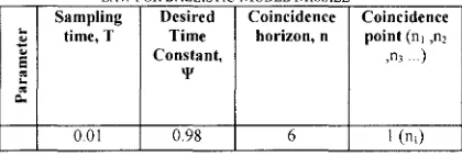
The missile moving scenario is set to be its reference trajectory of the missile mission. For this implementation, the scenario is developed by turning of missile up to 3 radians per second and turning it back at 2 radians per second before coming back to its original location. Using the PFC control law developed from Equation 2.7, the tuning parameters of PFC control law are stated in Table I below; TABLE I: PARAMETERS USED FOR DEVELOPED OF PFC CONTROL
LAW FOR BALLISTIC MODEL MISSILE
Sampling Desired Coincidence Coincidence
..
time, T Time horizon, n point (n 1 ,n2セ@
"
Constant, ,n, ... )E
"'
'I'..
"'
セ@
0.01 0.98 6 1 (n1)
From the result obtained in Figure 3, it shows that the output response follows the reference trajectory as the control output gives stable condition and found no ill-posed result. By observing the deflection of thrust chamber, the thrust chamber deflected shows some overshoot before quickly perform into the stable condition as the reference trajectory change its course. This condition is true for the chamber as it perform very fast turns to follow according to the reference trajectory. Overall result shows that the response is fast and quick to the stable
condition. Therefore, removal the prediction
mismatch is essential to improve the performance of PFC.
CONCLUSION & RECOMMENDATIONS
In conclusion, this paper has implemented a controller for an autopilot missile using Predictive Functional Control (PFC) method in state-space form, then coded to simulate using MATLAB 7 .0 environment. In all, based on the achievement/result the implementation of PFC algorithm seems intuitive and computationally simple. This truly important as the missile controller need not to be very complicated as it will explode as it reaches the target.
On the other hand, this section has also briefly shows that one can modify PFC so that it can handle
unstable system more reliably. It is a very good
motivation as any developments to extent would be useful. Also, as PFC is so simple to implement for fast system such as autopilot missile, this would be an opportunity for industries to exploit PFC.
This report tried to cover the main intent as more as possible. However this report does not mention how the PFC algorithm operates in nonlinear cases. Because of the limitation of the time this it was
not achievable. With clearly illustrated the
computation PFC model in Section III and its
170
implementation on Section IV, the idea of PFC methodology work on a fast system such as autopilot missile is explained.
Sometimes it is better to use a fast sampling rate (fast update of the receding horizon) with some prediction mismatch than to use slower sampling rate and less prediction mismatch. PFC allows the former, as it allows fast sampling rates. Moreover, due to the algorithm simplicity it is more straightforward to adapt for nonlinear models. Nonetheless, despite its apparent simplicity, PFC often gives very good performance, with constraint handling, quite similar to that achievable with a far more complex MPC algorithm.
ACKNOWLEDGMENT
Thanks are extended to all the colleague and staff
of Automatic Control & System Engineering
Department in the University of Sheffield, UK for their support in providing motivation and idea used for this project. Not forget from Universiti Teknikal
Malaysia Melaka (UTeM) for their strong
commitment towards academic excellence that encourages the researcher to go forward.
REFERENCE
[ 1] J. Richalet, "Pratique de la Commande Predictive." Editions Hermes, Paris, 1993.
[2] Clarke, D. W, Mothadi, C., & Tuffs, P. S.,"Generalized Predictive Control. Part I: the basic algorithm. Part II: Extensions and interpretations." Automatica, 23(2), pp.137-160, 1987.
[3] J A Rossiter,"Model-Based Predictive Control: A Practical Approach", CRC Press, 2003.
[4] E F Camacho and C Bordons,"Model Predictive Control", Springer, 2004.
[5] J.M Maciejowski, 2002. "Predictive Control With Constrains" Prentice Hall, 2002.
[6] J. B. Rawlings., "Tutorial Overview of Model Predictive Control. Special Edition: Industrial Process Control." IEEE Control Systems Magazine. pp 38-52, 2000.
[7] J. B. Rawlings, and K. R. Muske,"Stability of Constrained Receding Horizon Control". IEEE Transactions on Automatic Control. AC-38(10), 1512-1516, 1993 ..
"
[8) Muske, K.R and J.B. Rawlings, "Linear Model Predictive Control of Unstable Processes" J.Proc. Cont., 3(2), pp. 85-96, 1993.
[9] B. Kouvaritakis, J.A. Rossiter and AO.T Chang,"Stable Generalised Predictive Control: An Algorithm with Guaranteed Stability'', Proceedings IEE, Pt. D, 139(4), pp.349-262. 1992.
[image:5.598.34.244.205.276.2]APPENDIX 1 27 ft
E>o
68.5°TABLE II: CHARACTERISTICS AND COEFFICIENT OF d 3.75 ft
BASIC BALLISTIC MISSILE MODEL
q 585 lb/sqft
Altitude 36 000 ft
s
11.04 sg ftVelocity 1285 ft/sec d/(2U) mU/(Sq)
Cmq
- 0.321 sec88.5 sec
Mass 445 slugs
mg I (Sq)
-Cw
Cms
-Tl/(Sqd)2.22 -34.25
Iy 115 000 slug ft2
C,s
- T/(Sq) Iy I(Sqd) 4.75 sec2
- 4.63
c,.
- 3.13Cma
11.27....
--f', =U,, _ ... ···-·
ᄋセLセHMBO@---" LNNNセ@ Gセ|@
Horizontal
.---· ---· \
•
セコ@z,,
T
Figure 1: Ballistic missile axis system. [10]
The Thrust Chamber Deftect1on of The M1ss1le The Rate Change of Theta of The Missile
-5:
-10-セ@ -15
,§' ·20
-25-·30.
- - n 1 = 3 nh=6 n1=:10
·35
-0 0.2 0.4 0.6 0.8 1.2 1.4 1.6 1.8
Sampling T1me,t (sec)
0.9-
0.8-セ@
セ@
0.6-11 o.s,
I
0.4C
0.3·-
0.2'0.1
-0
0 0.2 0.4 0.6 0.8 1.2 Sampling Time,t (sec)
Figure 2: The Controller Response of the Computing Algorithm for'¥= 0.94
'
--- r, set-point
n1=3 n1:::6
n1=10
1.4 1.6 1.8
The Thrust Chamber Deflection of the Missile 2 The Rate Change of Theta of l'tle Missile
100
-0 2 6
Sampling Time,t (sec)
2.5-11.5
0 -0 1 2 3
Figure 3 The Missile Controller Response of the Ballistic Missile
Samphng Time.I (sec)
[image:6.595.41.464.48.730.2] [image:6.595.57.459.54.411.2] [image:6.595.30.463.365.700.2]