Mean Variance Optimal
VWAP Trading
∗
James McCulloch
†Vladimir Kazakov
‡May, 2011
Abstract
VWAP is the Volume Weighted Average Price of traded stock over a defined period. It is a metric of trade execution quality used by in-stitutional traders to minimize the execution cost of large trades. A riskless VWAP trading strategy is not possible without knowledge of final market volume. We formulate a mean-variance optimal VWAP strategy by assuming knowledge of final volume and then project this onto the space of strategies accessible to the VWAP trader. The mean variance optimal VWAP trading strategy is the sum of two distinct trading strategies, a minimum variance VWAP hedging strategy and a ‘directional’ price strategy independent of the hedging strategy and market VWAP. It is optimal for large volume VWAP traders to in-crease the size of the price ‘directional’ trade for additional return.
∗⃝c Copyright James McCulloch, Vladimir Kazakov, 2011. The authors thank Hardy Hulley for his invaluable suggestions, insights and criticisms. This paper is a draft: please do not quote without permission.
†Macquarie University, contact email: [email protected] ‡Quantitative Finance Research Centre (QFRC), University of Technology Sydney
1
Introduction
Volume Weighted Average Price (VWAP) trading is estimated to comprise 50% (2007 Bank of America Survey [26]) of all institutional trading and is used to minimize the execution costs of large trades in financial markets. This paper formulates a minimum mean-square (L2) VWAP trading strategy
which is then extended to a general optimal mean-variance strategy using the Markowitz [21] quadratic utility function.
For any institutional (large) trader the cost of trading is as important as the decision to trade. The cost of trading has three components: fees and commissions (generally fixed); the cost of execution; and opportunity cost. Execution cost (also known as ‘implementation shortfall’, Per´old [27]) is the difference in stock price between the time the decision to trade is taken and the eventual traded price. The major component of the execution cost is market impact cost, which is the adverse price movement due to the execution of a large trade on the market. Market impact cost results from the liquidity demand of large trades and information signalled to other market participants by the presence of a large trade in the market. Market impact cost can be reduced by fragmenting a large trade into smaller trades and spreading instantaneous liquidity demand over a longer trading period. Bertsimas and Lo [3] have formulated an optimal trade fragmentation schedule using a linear liquidity supply curve to model market impact.
Opportunity cost is foregone profit on volume that was not executed because of adverse price movement subsequent to the decision to trade. Op-portunity cost increases with time and since market impact cost decreases with time then total (execution + opportunity) transaction costs are convex in time. An optimal trading schedule based on a convex total transaction cost curve was formulated by Almgren and Chriss [1] using a market impact model that differentiates temporary and permanent adverse price movement due to liquidity demand.
The traded VWAP price compared to the VWAP price of all admissible trades1 over the same period was first proposed by Berkowitz, Logue and
Noser [2] as a benchmark of execution quality. They argue (page 99) that ‘a market impact measurement system requires a benchmark price that is an
1Not all trades are accepted as admissible in a VWAP calculation. Admissible trades are determined by market convention and are generally on-market trades. Off-market trades and crossings are generally excluded from the VWAP calculation because these trades are often priced away from the current market and represent volume in which a
‘randomly selected trader’ [2] cannot participate.
unbiased estimate of prices that could be achieved in any relevant trading period by any randomly selected trader’. They then define VWAP as an appropriate benchmark that satisfies this criterion. As with the optimal trading strategies of Bertsimas and Lo and Almgren and Chriss, a key feature of VWAP trading is the fragmentation of large trades into smaller trades in order to minimize market impact. The comparative studies of Domowitz and Yegerman [8] and Werner [37] show that the execution costs of VWAP are comparable to, or lower than, other block (large) trading strategies.
A non-adaptive optimal VWAP trading strategy fixed at the beginning of the VWAP period t = 0 (F0 adapted) has been formulated by Konishi
[19] for price modeled as a (martingale) Wiener process. We extend Kon-ishi’s formulation to a continuously updated dynamic mean-variance optimal VWAP strategy using the information available at time t (Ftadapted) with
price modeled as a continuous semimartingale. In addition, we show that the optimal VWAP trading strategies (eqn 16 and eqn 27) are closely associ-ated to the prediction of relative volume and minimize trading price impact by allocating trade volume (liquidity demand) during periods of maximum turnover (liquidity supply).
VWAP is naturally defined using relative volume Y rather than cumula-tive volumeV. The relative volume processY is defined as market cumulative volumeVtdivided by market total final volumeYt=Vt/VT and is adapted to
a filtration G which is the VWAP trader accessible (observed) filtration F
enlarged by knowledge of final volume Gt = Ft∨σ(VT). The VWAP price
VT (eqn 1) at time T can be formulated as an Itˆo integral under G with a
continuous price X integrator and with aG-predictable relative volume
pro-cess integrand ξtV,G = 1−Yt− . No zero risk F adapted (trader accessible)
VWAP trading strategy exists (lemma 3.7).
VT = X0 + ∫ T
0
ξV,G dX (1)
TheF adapted mean square optimal VWAP trading strategy is derived:
ξV,F
= min
ξF E
[ ( ∫ T
0 (
ξF
− ξV,G)
dX
)2]
(2)
This is then extended by deriving the F adapted Markowtiz
ξV,λ,F = max
ξF
[
E
[ ∫ T
0 (
ξF − ξV,G)
dX
]
− λ 2Var
[ ∫ T
0 (
ξF − ξV,G)
dX
] ]
(3)
The optimal mean variance VWAP trading strategy ξV,λ,F
is the sum of two distinct trading strategies, a minimum variance VWAP hedging strategy λ → ∞; ξV,∞,F
and a ‘directional’ price strategy ξ1
0 independent of the
hedging strategy and market VWAP. The ‘directional’ price strategy uses the properties of the Variance Optimal Martingale Measure (VOMM) to determine additional variance and expected return (section 3.3.2).
ξV,λ,F = ξV,∞,F + ξ
1,F
0
λ (4)
This is a general result, see McCulloch [23] for details. Any mean-variance hedging strategy (including VWAP) can be formulated as the sum of two con-ceptually and mathematically different trades, a minimum variance hedging strategy and an independent price ‘directional’ strategy. The price ‘direc-tional’ strategy is only dependent on the stochastic characteristics (VOMM) of the price process X. Furthermore, the additional variance of the opti-mal mean-variance solution is a direct sum of the minimum variance hedging strategy variance and the variance of the price ‘direction’ strategy. Simi-larly, the additional expectation of the optimal mean-variance solution is a direct sum of the minimum variance hedging strategy expectation and the expectation of the price ‘direction’ strategy (eqns 24 and 25).
Finally, a VWAP trader with aβVT trade size has a risk aversion
param-eter of (1−β)λ(section 3.3.3). Whereλis the trader risk aversion parameter for a small VWAP (β << 1) trade size. Thus it is optimal for large 0< β <1 mean-variance VWAP traders to increase the size of the price ‘directional’ trade for additional return.
ξV,λ,F = ξV,∞,F + ξ
1,F
0
2
Modelling VWAP
2.1
Price and Volume
Assumption 2.1.
(i) The stochastic environment of the VWAP asset is endowed with a stochas-tic basis(Ω,FT,F,P)with a standard (right continuous and complete)
filtration F ={Ft}0≤t≤,T. The filtration F contains all VWAP trader
accessible (observable) information about the VWAP asset. In addi-tion, the price process X is assumed to be aF continuous square
inte-grable semimartingaleX ∈ S2(P,F)and the cumulative volume process
V ∈ S2(P,F) is also a F square integrable semimartingale.
(ii) VWAP trading is normally conducted on single financial market assets. Therefore the exposition will assume univariate price X and cumulative volume V processes.
2.1.1 Final Volume, Relative Volume and the Initially Enlarged Filtration
Final volume is a square integrable positive integer valued random variable, VT ∈ L2(Ω,FT,P) (abbreviated VT ∈ L2(P)). A finite set of possible final
volumes exists VT ∈ SV, where the minimum element is the VWAP final
volume vT = min[v ∈SV] (no other market participants trade in the VWAP
period) and the maximum element is bounded, max[v ∈SV]<∞.
The filtrationG is the VWAP trader accessible filtration F initially
en-larged by the sigma algebra generated by final volumeσ(VT). Since VT isFT
adapted then FT =GT and it is a standard filtration underP. The enlarged
filtration G is formally defined as:
Gt = ∩
ϵ>0 (F
t+ϵ ∨ σ(VT)
Remark 2.2. Since the sigma algebra σ(VT) of final cumulative volume is
finitely large, the F semimartingale price processX is also aG
semimartin-gale (Jacod [16]).
Assumption 2.3. The price process X is a strictly positive continuous square integrable semimartingale with respect to the enlarged filtration G,
X ∈ S2(P,G).
The relative volume process is progressive cumulative volume divided by the final cumulative volume.
Yt =
Vt
VT
t∈[0, T] (6)
Relative volume is zero at time zero Y0 = 0, non-decreasing and has a
value of 1 at time T, YT = 1. It is measurable with respect to the enlarged
filtration G and is a square integrable semimartingale Y ∈ S2(P,G).
2.2
A Continuous Time Model of VWAP
One the reasons for the popularity of VWAP as a measure of order execution quality is the simplicity of its definition - the total value of all admissible trades divided by the total volume of all admissible trades. If Xi and ∆Vi
are the price and volume respectively of the ith trade in the VWAP period [0, T] withNT total trades, then the VWAP priceVT calculated at timeT is
readily computed as:
VT =
total traded value total traded volume =
∑NT
i=1 Xi∆Vi ∑NT
i=1 ∆Vi
Alternatively, the definition of VWAP can be written in continuous time notation. The price process X is a G semimartingale (remark 2.2), therefore
VWAP can be formulated as a G adapted Itˆo integral.
VT =
total traded value total traded volume =
1 VT
∫ T
0
0 0.2 0.4 0.6 0.8 1
10:00 11:00 12:00 13:00 14:00 15:00 16:00
Relative Volume Executed
Example Stock Intraday Relative Volume Trajectories
Mean
SUS TXT TXN
0 0.2 0.4 0.6 0.8 1
10:00 11:00 12:00 13:00 14:00 15:00 16:00
Relative Volume Executed
Example Stock Intraday Relative Volume Trajectories
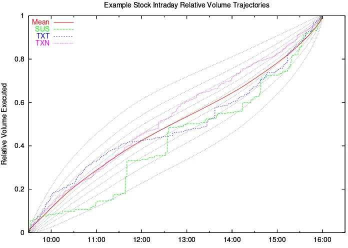
Figure 1: This graph shows an example of relative volume trajectoriesYt for
3 stocks representing low, medium and high turnover stocks. The red line is the expected relative volumeE[Yt] for all stocks trading more than 50 trades
a day on the NYSE. This expectation is the integral of the ‘U’ shaped trading intensity (dE[Yt]/dt) found on all major stock markets. SUS isStorage USA,
TXT isTextron Incorporated andTXN isTexas Instruments; on 2 July 2001 these stocks recorded 101, 946 and 2183 trades correspondingly.
Examining the integral above, it is readily seen that it relates to the relative volume processYt =Vt/VT. This is a key insight;VWAP is naturally
defined using relative volume Yt rather than actual volume Vt.
VT =
1 VT
∫ T
0
X−dV =
∫ T
0
X−dY
Integration by parts gives:
VT = XTYT − X0Y0 − ∫ T
0
Y−dX −
[
X, Y]
T
quadratic covariation term is zero [X, Y] = 0. Also Y0 = 0 and YT = 1 by
definition, so the integration by parts equation simplifies to:
VT = XT −
∫ T
0
Y−dX = X0 +
∫ T
0 (
1 − Y−
)
dX
Defining the G predictable integrand:
ξtV,G = 1 − Yt− = 1 −
Vt−
VT
(8)
Using this definition, VWAP has the following Itˆo integral representation:
VT = X0 + ∫ T
0
ξV,G dX
Remark 2.4. Note that unlike a conventional trading strategy where the constant term represents initial trading capital, the X0 term above (eqn 1) is
initial stock price and cannot be specified by a VWAP trader. Consequently, this constant term plays no role in optimizing VWAP trading strategies.
Since the price process is square integrable by assumption and the relative volume process is bounded by 1 (0 ≤ Yt ≤ 1), the VWAP random variable
3
Optimal VWAP Trading Strategies
It is shown (lemma 3.7) that VWAP is not attainable (Schweizer [34]) in the VWAP trader accessible filtration F and any feasible F adapted
trad-ing strategy is risky. Therefore the objective is to specify a feasible mini-mum risk F adapted VWAP strategy and extend this to a Markowtiz
mean-variance optimal strategy. This is an application of the theory of the optimal quadratic projection of random variablesH ∈L2(P) onto a subspace of Itˆo
in-tegrals (ξ·X)T ∈L2(P). The extensive quadratic hedging literature includes
Chunli and Karatzas [15], Schweizer [34] [35], Delbaen and Schachermayer [7], Rheinl¨ander and Schweizer [31], Pham and Rheinl¨ander and Schweizer [28], Gouri´eroux and Laurent and Pham [13] and Rheinl¨ander [30].
Optimal VWAP trading belongs to the class of hedging problems where the accessible filtrationF is smaller than the filtrationG required for hedge
replication to be attainable. This has been studied by Schweizer [32] for martingale X and has also been studied by F¨ollmer and Schweizer [10], who gave a solution that was local error minimizing for semimartingaleX. Møller [24] [25] and Schweizer [36] extended this to a Markowitz mean-variance optimal solution for semimartingale X.
This section formulates a minimum mean-square (L2) VWAP strategy
for martingale X, extends this to a mean-square (L2) optimal strategy for
semimartingale X (eqn 2) and finally develops a Markowitz mean-variance optimal VWAP strategy (λ≥0) for semimartingaleX (eqn 3).
3.1
Preliminaries
3.1.1 Existence of Equivalent Local Martingale Measures
The Itˆo integral with integrand ξ is notated:
GT(ξ) =
∫ T
0
ξ dX
LetL(X,G) denote the space of allX-integrable G predictable processes.
The set of admissibleG predictable integrands where the resulting integration
Θ(G) = {
ξG
∈L(X,G)(ξG ·X)t ∈ S2(P,G)}
Note that ξV,G
∈Θ(G) by definition. The set of signed local martingale
measures such that anyg ∈GT(Θ(G)) is a local martingale (these definitions
from Delbaen and Schachermayer [7]) are defined:
Ds(G) = {ZG ∈L2(Ω,FT,P)∀g ∈GT(Θ(G)), E[Z
G
g] = 0, E[ZG ] = 1}
Ms(G) = {
QG dQ
G
/dP=ZG , ZG
∈ Ds(G)}
From lemma 2.1 in Delbaen and Schachermayer [7] the set of signed lo-cal martingale measures Ds(G) ̸= ∅ is non-empty if the constant 1 is not
contained in GT(Θ(G)).
Assumption 3.1. 1∈/ GT(Θ(G)) and therefore Ds(G)̸=∅.
The set of equivalent local martingale measures is the subset of signed local martingale measures that are strictly positive and therefore probability measures.
De(G) = {
ZG ∈ Ds(G) Z
G >0}
Me(G) = {
QG dQ
G
/dP=ZG, ZG ∈ De(G)}
The sets of signed local martingale measures and equivalent local martin-gale measures are equal (De(G) =Ds(G),Me(G) =Ms(G)) if price process
X is G continuous (Delbaen and Schachermayer [7]). Therefore by
assump-tion 2.3 Me(G)̸=∅.
The proper subset (lemma 3.7) Θ(F) ⊂ Θ(G) is defined where all the
Θ(F) = {
ξF
∈L(X,F)(ξF ·X)t∈ S2(P,F)}
Finding the optimal mean square adapted strategyξF
is a Hilbert space projection from L2(P) onto G
T(Θ(F)). Therefore the closure of GT(Θ(F))
in L2(P) is a necessary property. The set of equivalent local martingale
measures such that any f ∈GT(Θ(F)) is a local martingale is defined:
Ds(F) = {
ZF ∈L2(Ω,FT,P)∀f ∈GT(Θ(F)), E[ZFf] = 0, E[ZF] = 1}
From the F continuity of X (assumption 2.1) the sets of signed local
martingale measures and equivalent local martingale measures are equal:
De(F) = Ds(F) (9)
Me(F) = {
QFdQ
F
/dP= ZF , ZF
∈ De(F)}
Since GT(Θ(F)) ⊂ GT(Θ(G)) it is intuitive and true that De(G) ⊆
De(F) andMe(G)⊆ Me(F) and therefore from assumption 3.1Me(F)̸=
∅.
3.1.2 Closure of the Itˆo Integral Subspaces
Definition 3.2. TheF Variance Optimal Martingale Measure (VOMM) is
defined as the equivalent local martingale measure Q˜F
∈ Me(F) such that
the associated density Z˜F
∈ De(F) has the minimum L2(P) norm:
dQ˜F
dP = ˜Z
F
= min
ZF∈ De(F)
Z
F
L2(P) = min
ZF∈ De(F)Var[Z F
Definition 3.3. A uniformly integrable strictly positive (P,F) martingale
Z > 0 satisfies the F reverse H¨older condition, denoted Z ∈ Rp(P,F), if
there is a constant C <∞ such that for every stopping time 0≤ τ ≤T the following relationship exists:
E
[ (
Z Zτ
)p
Fτ
]
≤C p∈(1,∞)
Assumption 3.4. The VOMM density Z˜F
satisfies the F reverse H¨older
inequality, Z˜F
∈ R2(P,F).
If theF VOMM density satisfies theF reverse H¨older inequality ˜ZF ∈ Me(F)∩ R
2(P,F), the closure of GT(Θ(F)) in L2(P) was proved by
Del-baen, Monat, Schachermayer, Schweizer and Stricker [6] (theorem 4.1).
3.2
L
2Optimal Strategies
3.2.1 An L2 Optimal Strategy for Martingale X
Let PG denote the predictable sigma field of G. The sigma finite Dol´eans
measure νQ and associated product space can be defined using continuous
square integrable local martingale X under any equivalent local martingale measure QG ∈ Me(G):
( Ω×[0, T], PG⊗B[0, T], νQ); νQ(A) =
∫
Ω ∫ T
0
1A(t, ω)d⟨X⟩t(ω)dQ
G (ω).
Let A = H ×B where H ⊆ PG and B ∈ B[0, T], the conditional
expectation of the product space is denoted:
ξA,Q = E⟨X⟩,Q[ξG | A]
Lemma 3.5. LetA=H ×B where H ⊆ PG andB ∈ B[0, T]. For anyPG
adapted process ξG
∈( Ω×[0, T], PG ⊗ B[0, T], ν
Q) the explicit time indexed
product space conditional expectation is formulated:
ξtA,Q = 1B(t)
Proof. Using the definition of conditional expectation, Fubini’s theorem and the definition of the σ-finite Dol´eans measure:
∫
Watanabe [20]) to the corresponding norm on L2(Ω,F
T,QG) and the
isom-The conditional expectation, ξF,Q
= E⟨X⟩,Q[ξG
|F ×[0, T] ] is the F
adapted process that minimizes the norm ∥ξG
−ξF,Q∥
L2(⟨X⟩,Q). Therefore it is immediately clear from the isometry thatξF,Q is theF adapted integrand
that minimizes ∥(ξG
3.2.2 VWAP is Not Attainable in the Observed Filtration
Definition 3.6. A random variable UT ∈L2(P) is F attainable (Schweizer
[34]) if a unique F adapted predictable process γU,F
exists such that UT is
replicated by the following Itˆo integral.
UT = U0 +
∫ T
0
γU,FdX
Lemma 3.7. VWAP is not F attainable.
Proof. By contradiction. Assume VWAP is F attainable and an attainable F predictable strategyξV,F
exists, then from eqn 1 and eqn 8 above:
VT =
∫ T
0
ξV,G dX =
∫ T
0
ξV,F dX
Hence for allQG ∈ Me(G) the product space isometry implies that:
∫ T
0
ξV,FdX −
∫ T
0
ξV,G dX
L2(Q)
= ξV,
F
− ξV,G
L2(⟨X⟩,Q) = 0
The equation above implies that ξV,G
= E⟨X⟩,Q[ξV,G
|F ×[0, T] ].
How-ever,ξV,G
= 1−Y−is notFtmeasurable for 0≤t < T because, by definition,
final cumulative volume VT (eqn 8) is not Ft measurable 0≤t < T.
There-foreξV,G
̸=E⟨X⟩,Q[ξV,G
3.2.3 An L2 Optimal VWAP Strategy for (Q,G) Martingale Price
The explicit product space conditional expectation (eqn 10 in lemma 3.5) can be applied to give the F mean square optimal trading strategy for VWAP
under any QG ∈ Me(G) in the associated Hilbert space L2(Ω,F
T,QG):
ξtV,F,Q = 1[0,T](t)E
Q[ξV,G
t d⟨X⟩t|Ft]
EQ[d⟨X⟩
t|Ft]
= EQ[ξtV,G |Ft] (11)
In particular, if P ∈ Me(G) and price X is a (P,G) martingale, the F
L2 optimal strategy is also the minimum variance strategy2:
ξtV,F = 1 −
Vt
E[VT |Ft]
(12)
Remark 3.8. If price X is a (P,G)martingale, then the minimum variance
VWAP strategy depends on the prediction at time t < T of final volume VT.
3.2.4 An L2 Optimal Strategy for Semimartingale X
This section is based on the theory of optimal L2 hedging for continuous
semimartingale processes. The main results of the extensive literature (sum-marized in Schweizer [35]) are sketched below.
Using the F VOMM density ˜ZF
, the process ˆZF
t can be defined as
follows:
ˆ
ZtF = EQ˜
[
dQ˜F dP
Ft
]
= E[ ( ˜Z F
)2|F
t]
E[ ˜ZF|F
t]
(13)
There exists an integrandζF
∈ Θ(F) (lemma 2.2 Delbaen and
Schacher-mayer [7]) such that the process ˆZF
can be expressed as the integral:
ˆ as the ˜QF conditional expectation ofH:
WtH,F,Q˜ = EQ˜[H Ft
]
The Galtchouk [12], Kunita and Watanabe [20] (GKW) decomposition of martingale WH,F,Q˜
with respect to martingale X under VOMM ˜QF can be formulated:
square integrable martingale strongly orthogonal to X under ˜QF
. Finally, the mean square optimal integrand ξH,F
for H under P is given by the following feedback equation:
ξtH,F = ξtH,F,Q˜ − ζ
3.2.5 An L2 Optimal VWAP Strategy for Semimartingale X
The VWAP constant term X0 (initial stock price) cannot be modified by
the VWAP trader (remark 2.4). Therefore it is VT −X0 (the Itˆo integral
WtV,F,Q˜ = E
The orthogonal martingaleLV,F,Q˜ is the F measurable difference:
LVt,F,Q˜ =
Substituting this into equation 15 gives the mean square optimal feedback solution (trading strategy) for VWAP trading with semimartingale X (ζF
t is
The mean square optimal VWAP trading strategy equation has an intu-itive interpretation. The first term of the equation, the GKW decomposition of the martingale EQ˜[V
T −X0|Ft], is the approximation to the P optimal
strategy under the ‘closest’ F adapted equivalent local martingale measure
˜
QF
. The second term is a feedback error correction term based on updating the accumulated strategy error in the time interval [0, t] using the available information at time t. It is also clear that the prediction EQ˜[ξV,G
t |Ft] is
central to the ‘practical’ implementation of the optimal strategy, and since cumulative volume Vt is F adapted, this is equivalent (eqn 8) to the
pre-diction of final volume EQ˜[V
T|Ft]. Under the restrictive assumption that
price X and final volume VT are independent (see section 3.4.2) the
opti-mal solution simplifies to the P prediction E[VT|Ft]. A dynamic prediction
3.3
Mean Variance Optimal VWAP Strategies
For a more general and detailed treatment of the material in this section refer to McCulloch [23].
3.3.1 The Minimum Variance VWAP Strategy
The VOMM density ˜ZF
is closely related to the complement of the pro-jection of the constant 1 onto GT(Θ(F)). Define closed subspace K =
span{1, GT(Θ(F))} ⊂ L2(P). Then the VOMM density ˜ZF ∈ K and is
the normalized projection of the constant 1 onto GT(Θ(F))⊥.
If the operator π is defined as the projection operator from L2(P) onto
the orthogonal complement GT(Θ(F))⊥ and ξ1,F ∈ Θ(F) is the integrand
of the projection of 1 onto GT(Θ(F)), then:
˜ ZF
= π(1)
E[
π(1)] =
1
E[
π(1)] − ∫ T
0
ξ1,F
E[π(1)]dX (17)
From E[π(1)] =E[π(1)2] and the definition above:
Var[ ˜ZF] = 1
E[π(1)] − 1 (18)
The minimum variance (λ → ∞ in eqn 3) VWAP strategy ξV,∞,F (see McCulloch [23], eqn 6) is the sum of the L2 optimal strategy ξV,F
and the constant weighted integrand of the projection of 1 onto GT(Θ(F)):
ξV,∞,F = ξV,F − (
Var[ ˜ZF] + 1)
E
[ ∫ T
0 (
ξV,G − ξV,F)
dX
]
ξ1,F (19)
Using the definition of the VOMM ˜QF
E
3.3.2 The Mean Variance Optimal VWAP Strategy
If the price process is semimartingale under the observed filtration F, then
the trader may wish to exploit expected price movement to ‘beat’ VWAP. A trader can exploit expected price movement for the benefit of his client by adopting a VWAP trading strategy that is riskier than the minimum variance strategy in return for a positive expected return. The optimal mean-variance VWAP trading strategy is derived using the Markowitz quadratic mean-variance utility function (eqn 3) with a risk aversion coefficient 0 ≤ λ < ∞. The mean-variance optimal strategy ξV,λ,F
can be formulated [23] as the sum of two distinct trading strategies, a minimum variance VWAP hedging strategy λ→ ∞; ξV,∞,F
and a standard ‘directional’ price strategy ξ1
0 independent of the hedging strategy and market VWAP:
ξV,λ,F = ξV,∞,F + ξ
1,F
0
λ (22)
Where the independent standard (λ = 1) mean-variance optimal price ‘directional’ trade is formulated:
ξ01,F = (
Var[ ˜ZF
] + 1)
ξ1,F
The increases in expected return and variance for an optimal mean vari-ance VWAP trading strategy are proportional to the varivari-ance of the density
of the F VOMM:
3.3.3 Mean Variance Risk Aversion λ and VWAP Trade Size
The greater the proportion of total trading that the VWAP trader controls, the easier it is to trade at the market VWAP price. In the limiting case, the trader controls all traded volume and exactly determines the market VWAP irrespective of trading strategy. Thus VWAP risk is proportional to the traded volume that the VWAP trader does not control.
The market relative volume processY can be written as a weighted sum of the relative volume of other market participants ¯Yt= ¯Vt/V¯T and the relative
volume strategy of the VWAP trader yt = vt/vT. The proportion β of the
total market volume traded by the VWAP trader is then calculated:
β = ¯ vT
VT +vT
= vT VT
0< β≤1
The total relative volume can now be decomposed into the relative volume process of other market participants ¯Yt and the relative volume strategy of
the VWAP trader yt.
Yt = (1−β) ¯Yt + βyt
VT = X0 + (1−β)
Therefore if the VWAP trader final volumevT is fixed and the final volume
of other market participants ¯VT cannot be influenced by the VWAP trader,
then the proportion of total volume VWAP traded β cannot be optimized (by increasing β). The mean square error of the VWAP trading strategy is specified:
It is also readily shown that variance of the VWAP trading strategy is also scaled by (1−β)2 and expected return by (1−β). Hence, including
the VWAP traded volume proportion into the mean variance optimization in equation 3 is equivalent to reducing the risk aversion parameter λ by a factor of (1−β):
Thus a VWAP trader with aβVT trade size and risk aversion λ has then
same mean variance optimal strategy as a VWAP trader with small (β << 1) trade size with risk aversion parameter (1−β)λ. It is interesting to note that β is a random variable in filtration F and the specification of risk aversion
is uncertain in the VWAP trader information set.
Remark 3.9.
(i) The optimal mean square (eqn 16) and minimum variance (eqn 19) VWAP strategies (λ → ∞) are unchanged by VWAP trade size.
(ii) A VWAP trader with a βVT trade size has a risk aversion parameter
ξV,λ,F
= ξV,∞,F
+ ξ
1,F
0
(1−β)λ
3.4
Simplifying Assumptions For VWAP Strategies
The optimal mean variance VWAP strategies (eqns 16, 19, 22 and 5) allow generality in specifying the VWAP asset price process X and the nature of the dependence between price X and final volume VT (the relationship
be-tween filtrationsF andG) but at the cost of the strategies being formulated
at an abstract level. Since VWAP is a ‘practical’ trade, it is worthwhile dis-cussing restrictive assumptions on the price process and the (in)dependence between price and final volume in order to simplify the specification of the optimal VWAP strategies. Finally, as an example, we specify an optimal mean variance VWAP strategy using price modeled as a geometric Brownian motion (GBM) with final volume and price assumed to be independent.
3.4.1 The VOMM and Minimal Martingale Measure Coincide
It is clear from the form of the optimal VWAP strategies that an explicit formulation of the density ˜ZF
of the F VOMM is required. In practice, the F VOMM is usually not known and is difficult to formulate (Heath, Platen
and Schweizer [14]). However, if the price process satisfies thestructure con-dition and the resultant mean-variance tradeoff process is deterministic at timeT thenF VOMM coincides with the readily formulated minimum
mar-tingale measure (Schweizer [33], Schweizer [35] and F¨ollmer and Schweizer [11]). Briefly, the (continuous) price process satisfies the structure condition if the drift term Aof the canonical decomposition under Pis absolutely con-tinuous with respect to the predictable quadratic variation of the martingale M:
Xt = X0 + Mt +
∫ t
0
α d⟨M⟩
Kt =
If KT is deterministic then the minimum martingale measure (MMM)
density, ˇZF
Using the VOMM and MMM equivalence, the generalized Bayes formula and lemma 4.7 in Schweizer [35], the abstract form of the L2 optimal VWAP
trading strategy (eqn 16) is simplified to:
ξtV,F =
We remark that if the VOMM is equivalent to the MMM then explicit mean-variance optimal price ‘directional’ strategies are readily formulated, see McCulloch [23] for details.
ξ01,F = αtE
3.4.2 The Independence of VT and X
The assumption of the independence of final volumeVT and priceXsimplifies
the form of the optimal VWAP strategy. Under the independence assump-tion, the canonical decomposition ofX =M+Ais unchanged underG (thm
2 page 364, Protter [29]). Therefore, invoking Girsanov’s theorem, for any
QF ∈ Me(F) priceX is a (QF
,G) martingale and hence QF
∈ Me(G).
However, price andcumulativevolumeVtare considered to be interrelated
accessible) process that is the difference between cumulative buyer initiated volume (volume traded at the ask price) and cumulative seller initiated vol-ume (volvol-ume traded at the bid price) and is influential on price direction (Chan, Chung and Fong [5]). The dependence of final volume VT and price
X will be weaker than signed volume since final volume does not contain any obvious price directional information. Nonetheless, the assumption that final volume VT is independent of price X is restrictive.
Under the assumption of independence, ˜ZF
∈ De(G) is a (P,G)
martin-gale and is Ft adapted:
EQ˜[ξtV,G |Ft] = E[ ξ
Therefore theL2 optimal VWAP trading strategy (eqn 16) is simplified:
ξtV,F = E[
,G) martingale then the mean-square and
min-imum variance solutions coincide ξV,F
= ξV,∞,F
and the expectation of the minimum variance VWAP strategy (eqn 20) is zero:
EQ˜
3.4.3 Mean Variance VWAP with GBM
Finally, we conclude this section with an example of mean variance optimal VWAP where the price process is assumed to be a Geometric Brownian Motion (GBM), a continuous semimartingale commonly used to describe the price process on financial markets. The GBM satisfies the structure condition and is usually specified as a stochastic differential equation:
dXt = µ Xtdt + σ XtdWt
where Wt is a standard Brownian motion and µ and σ are constants.
Hence, the mean-variance tradeoff process is deterministic and the VOMM and MMM coincide:
αt =
µ σ2X
t
, Kt =
µ2
σ2 t
˜
ZtF = ˇZtF = exp
(
−µ
σ Wt −
1 2
µ2
σ2 t )
If we further assume that final volume VT and price X are independent,
then the minimum variance optimal VWAP trade is formulated:
ξtV,∞,F = E[ξtV,G |Ft] + µ
σ2X
t
∫ t
0 (
E[ξsV,G |Ft] − ξV,F
s
)
dXs (28)
We emphasize that the key to the practical and efficient implementation of this simplified VWAP algorithm is the prediction of final volume VT given
the available information Ft at time t:
E[ξtV,G |Ft] = 1 − Vt
E[VT |Ft]
To complete the mean-variance optimal GBM example, we assume that the VWAP trader is tradingβVT of total market volume in the VWAP trade
ξV,λ,F
= ξV,∞,F
+ ξ
1,F
0
(1−β)λ
ξ01 = µ
σ2X
t
(
Xt
X0
)−µ/σ2
exp
( (µ
σ2 −1 )µt
2
)
4
Conclusion
We consider a continuous time model of optimal VWAP trading and derive optimal Markowitz mean-variance VWAP trading strategies. These results generalize Konishi’s [19] fixed F0 adapted solution for a martingale Wiener
process price to a continuously dynamic Ft adapted solution for continuous
semimartingale price. In addition, we show that the optimal VWAP trad-ing strategies (eqn 16 and eqn 27) are closely associated to the prediction of relative intraday volume (E[Yt|Ft]) and minimize trading price impact
References
[1] Robert Almgren and Neil Chriss, Optimal execution of portfolio trans-actions, Journal of Risk 3 (2000), 539.
[2] Stephen Berkowitz, Dennis Logue, and Eugene Noser, The Total Cost of Transactions on the NYSE, Journal of Finance 43 (1988), 97–112.
[3] Dimitris Bertsimas and Andrew Lo,Optimal Control of Execution Costs, Journal of Financial Markets 1 (1998), 1–50.
[4] Jedrzej Bia lkowski, Serge Darolles, and Ga¨elle Le Fol,֒ Improving VWAP strategies: A dynamic volume approach, Journal of Banking & Finance
32 (2008), 1709–1722.
[5] Kalok Chan, Y. Peter Chung, and Wai-Ming Fong, The Informational Role of Stock and Option Volume, Review of Financial Studies15(2002), 1049–1075.
[6] Freddy Delbaen, Pascale Monat, Walter Schachermayer, Martin Schweizer, and Christophe Stricker, Weighted Norm Inequalities and Hedging in Incomplete Markets, Finance and Stochastics1(1997), no. 3, 181–227.
[7] Freddy Delbaen and Walter Schachermayer,The Variance-Optimal Mar-tingale Measure for Continuous Processes, BERNOULLI 2 (1996), 81– 105.
[8] Ian Domowitz and Henry Yegerman, The Cost of Algorithmic Trading: A First Look at Comparative Performance, Algorithmic Trading: Preci-sion, Control, Execution. (Brian R. Bruce ed.) (2005), 30–40.
[9] Thomas W. Epps, Security Price Changes and Transaction Volumes: Theory and Evidence, The American Economic Review65(1975), no. 4, 586–597.
[10] Hans F¨ollmer and Martin Schweizer, Hedging of Contingent Claims un-der Incomplete Information, Applied Stochastic Analysis (M.H.A. Davis and R.J. Elliot eds) (1991), 389–414.
[12] Leonid Galtchouk, Repr´esentation des martingales engendr´ees par un processus `a accroissements ind´ependants (cas des martingales de carr´e int´egrable), Annales de l’Institut Henri Poincar´e (B)12(1976), 199–211.
[13] Christian Gouri´eroux, Jean-Paul Laurent, and Huyˆen Pham, Mean-variance hedging and num´eraire, Mathematical Finance 8 (1998), 179– 200.
[14] David Heath, Eckhard Platen, and Martin Schweizer, A Comparison of Two Quadratic Approaches to Hedging in Incomplete Markets, Mathe-matical Finance 11 (2001), 385–413.
[15] Chunli Hou and Ioannis Karatzas, Least-Squares Approximation of Ran-dom Variables by Stochastic Integrals, Advanced Studies in Pure Math-ematics; Stochastic Analysis and Related Topics in Kyoto - In Honour of Kiyosi Ito; Edited by Hiroshi Kunita, Shinzo Watanabe, Yoichiro Takahashi 41 (2004), 141–166.
[16] Jean Jacod, Grossissement Initial, Hypoth`ese (H’) et Th´eor`eme de Gir-sanov, S´eminaire de Calcul Stochastique 1982/83, Lecture Notes in Mathematics 1118, Springer (1985), 15–35.
[17] Prem C. Jain and Gun-Ho Joh, The Dependence between Hourly Prices and Trading Volume, Journal of Financial and Quantitative Analysis23
(1988), 269–283.
[18] Jonathan M. Karpoff, A Theory of Trading Volume, The Journal of Finance 41 (1986), no. 5, 1069–1087.
[19] Hizuru Konishi, Optimal slice of a VWAP trade, Journal of Financial Markets 5 (2002), 197–221.
[20] Hiroshi Kunita and Shinzo Watanabe,On square integrable martingales, Nagoya Mathematical Journal 30 (1967), 209–245.
[21] Harry Markowitz, The optimization of a quadratic function subject to linear constraints, Naval Research Logistics Quarterly (1956), no. 3.
[22] James McCulloch, Relative Volume as a Doubly Stochastic Binomial Point Process, Quantitative Finance7 (2007), 55–62.
[24] Thomas Møller, Indifference Pricing of Insurance Contracts: Theory, Working Paper no. 170, Laboratory of Actuarial Mathematics, Univer-sity of Copenhagen, February 2001.
[25] , Indifference pricing of insurance contracts in a product space model, Finance and Stochastics 7 (2003), 197–217.
[26] Bank of America, Marching up the Learning Curve: The Second Buy-Side Algorithmic Trading Survey, February 2007.
[27] Andre F. Per´old, The Implementation Shortfall: Paper versus Reality, The Journal of Portfolio Management 14 (1988), 4–9.
[28] Huyˆen Pham, Thorsten Rheinl¨ander, and Martin Schweizer, Mean-variance hedging for continuous processes: New proofs and examples, Finance and Stochastics 2(1998), 173–198.
[29] Phillip Protter, Stochastic Integration and Differential Equations, Springer, 2005.
[30] Thorsten Rheinl¨ander, Optimal martingale measures and their appli-cations in mathematical finance, Ph.D. thesis, Technische Universit¨at Berlin, 1999.
[31] Thorsten Rheinl¨ander and Martin Schweizer, On L2-projections on a
space of stochastic integrals, Annals of Probability25(1997), 1810–1831.
[32] Martin Schweizer, Risk-minimizing hedging strategies under restricted information, Mathematical Finance4 (1994), 327–342.
[33] ,On the Minimal Martingale Measure and the F¨ollmer-Schweizer Decomposition, Stochastic Analysis and Applications 13 (1995), 573– 599.
[34] , Approximation Pricing and the Variance-Optimal Martingale Measure, Annals of Applied Probability 24 (1996), 206–236.
[35] , A guided tour through quadratic hedging approaches, Option Pricing, Interest Rates and Risk Management (E. Jouini, J. Cvitanic, and M. Musiela, eds., Cambridge University Press, 2001.
[36] , From Actuarial to Financial Valuation Principles, Insurance: Mathematics and Economics 28 (2001), 31–47.