P
Revisited: Money-Based Inflation
Forecasts with a Changing Equilibrium
Velocity
Athanasios Orphanides and Richard D. Porter
Alternate recursive estimates of equilibrium velocity are obtained by applying regression trees and OLS methods to a standard representation of M2 demand. Equilibrium velocity is defined as the velocity level that would be expected to hold if deposit rates were at their long-run average (equilibrium) value. We simulate the alternative models to obtain real-time forecasts of inflation and evaluate the performance of the forecasts obtained from the alternative models. While a P*model based on a constant equilibrium velocity does not provide accurate inflation forecasts over the 1990s, we find that a model based on our time-varying equilibrium velocity estimates is quite accurate. © 2000 Elsevier Science Inc.
Keywords: Inflation forecasting; M2 velocity; Quantity equation
JEL Classification System: E30; E50
I. Introduction
Given an estimate of real potential output, Q*, and an estimate of equilibrium velocity, V*, P*is defined as the equilibrium level of prices supported by the current quantity of money in circulation, M:
P*;
MV*
Q* (1)
As Hallman et al. (1991) showed, P*can potentially provide a useful anchor for the price level and as such be utilized as a tool for predicting inflation. The framework for understanding the monetary dynamics of inflation relies on the simple idea that if the
Division of Monetary Affairs, Board of Governors of the Federal Reserve System, Washington, D.C. Address correspondence to Dr. Richard D. Porter, Federal Reserve Board, Stop 72, Washington D.C. 20551.
current price level, P, deviates from its equilibrium level, P*, then inflation will tend to move so as to close this gap between the actual and equilibrium price levels—the price gap.
However, implementation of the framework requires a firm understanding of what the level of equilibrium velocity is. Much of the original appeal of the Hallman et al. study was based on the simplicity of their definition of V*. Using the M2 monetary aggregate, they showed that assuming a constant equilibrium velocity for their sample (1955–1988) was a sufficiently accurate representation despite the waves of financial innovation, which had taken place during that time period. As monetary practitioners and theorists have always recognized, however, continuous innovation in financial markets implies that such presumed observed constancies cannot be taken for granted.1
By now, it is well known that the presumption of constancy of the equilibrium velocity of M2 is no longer valid. As early as 1991 the stability of the historical statistical relationships involving M2 was already being questioned at the Board of Governors. [See Feinman and Porter (1992) for an early accounting of this breakdown. Orphanides, Reid and Small (1994) discuss the role of financial innovation in this breakdown.] And consequently, it was recognized that using the P*framework to forecast inflation, based on the assumption of a constant equilibrium velocity for M2, was no longer reliable.
In this paper we investigate how to adapt the original P*framework to an environment in which V*may be time varying. Specifically, we provide some guidance regarding how the equilibrium velocity of M2 could be adjusted in real time to enable continuing use of the price gap for forecasting inflation.
An obvious ex post “correction” could been obtained directly by simply computing the value of V* that would have eliminated the inflation forecast errors resulting from the incorrect assumption of a constant V*. But such an exercise is circular and would be useless for forecasting inflation in real time. Rather, information from other variables observed contemporaneously with velocity should be brought into consideration. To that end, we examine the co-movements of velocity and the opportunity cost of money suggested from traditional money demand formulations as our alternative source of information regarding potential changes in equilibrium velocity and compute the change in V*implied in that relationship.2We examine several alternative specifications of V*that could have reasonably been obtained in real time by recursive estimation, as soon as the breakdown in equilibrium velocity was recognized. Eventually, each of our estimates exhibits a noticeable upward shift in equilibrium velocity of about the same amount, although they differ somewhat regarding the date when the shift became evident.
Using these alternative specifications of V*we then show the corresponding 1-year-ahead inflation forecasts for the 1990s. The results suggest that much of the deterioration in the inflation forecasts obtained from the P*framework using the incorrect assumption of constant equilibrium velocity is reversed once we account for the apparent shift in equilibrium velocity.
1Indeed, in recognition of this truism, Hallman et al. warned that “[if] permanent shifts to velocity are
empirically significant, actual prices would diverge from P*in the long run.”
2Koenig (1994) recognized the usefulness of bringing information from such sources to bear on the P*
framework when he proposed a simultaneous estimation of money demand and P*models.
II. Equilibrium Velocity
Traditional theories for the demand for money posit that velocity fluctuates with the opportunity cost of money. Letting ˜ denote deviations of the opportunity cost ofOC money, OC, from its average norm, a simple way to capture this relationship is as follows:
V5V*1a1˜OC1e (2)
where a1 measures the response of velocity to movements in the opportunity cost of money and e is a stationary zero mean error term. In this setting the stability of V*can be examined in a straightforward manner. If V*were a constant, it could be easily estimated from the (population) regression: where, of course, an estimate of V*could be obtained as the estimated intercept parametera0in this regression:
V5a01a1˜OC1e (3)
Hallman et al. implicitly relied on the stability of money demand and the absence of any trend in the movement of˜ over the sample period in which they developed the POC * model. Specifically, if in the above population regression the error term, e, averages about zero and departures of OC from its norm, ˜, also average about zero, then it isOC immediate from this regression that the sample mean of V, V#, will give a good estimate of V*, which is the estimate that Hallman et al. selected. However, if V*shifts up, as it apparently has in the early 1990s, the revised estimate of V*needs to embody some of the upward drift of the velocity error e, which occurred then.
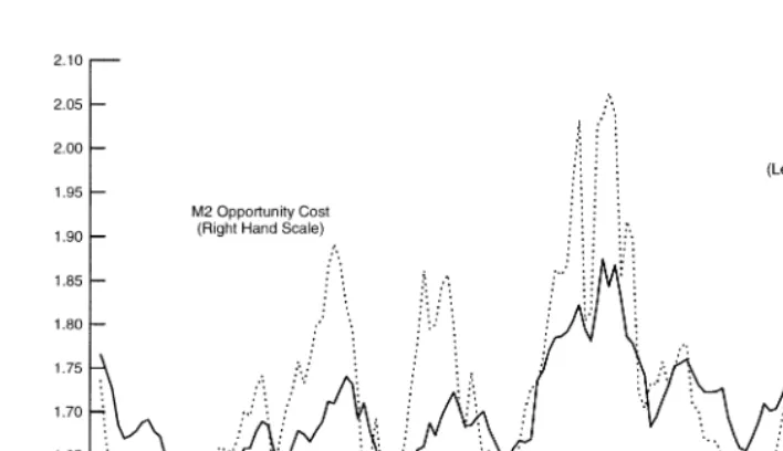
Defining the opportunity cost of M2 holdings as the rate on the 3-month Treasury bill minus the average rate paid on M2 balances, the relationship between M2 velocity and the opportunity cost is shown in Figure 1.3As can be seen, between 1960 and until about 1990, M2 velocity and opportunity cost moved together quite closely and could likely be
3See the data appendix for details on the definitions.
described by the simple regression above. Indeed, the relationship implicit in this diagram has formed the basis for models of M2 demand, including the models in Moore et al. (1990), which were used at the Board of Governors for the last decade.4Since about 1990, however, the gap between M2 velocity and opportunity costs widens in a way that does not appear to fit the previous relationship.
Figure 2 provides a scatter plot of the same data. The solid line shows the regression line of velocity on the opportunity cost estimated with data from 1960:1 to 1988:4. The two dotted lines form a 95 percent confidence band for the fitted values of velocity. As can be seen, the assumption of a constant V*for this period is not incompatible with this model. The point estimate for V*can be read as the value of the fitted line corresponding to the historical norm of the opportunity cost. Starting in about 1991, however, the observed velocity of M2 is consistently outside the confidence band obtained based on the assumption of a constant V*. These results suggest that by 1991, the constancy of V*should have been seriously questioned—as was indeed the case.
Unlike Hallman et al., who posit that V*is a constant, however, money demand models including Moore et al. typically allow for the possibility of a trend in V*. This can be easily captured by specifying
V5a01a1˜OC1a2TIME1e (4)
where V*5a01a2TIME. As it turns out, a small positive trend does appear in the data. Although statistically significant, it is very small compared to the movements of velocity after 1991. Consequently, the possible omission of a trend in computing V* cannot by itself account for the apparent non-constancy of equilibrium velocity. Nonetheless, for later comparisons, we will use both formulations including and excluding a trend as benchmarks.
4Figure 1 is in essence an updated and rescaled version of Figure 9 in Moore et al. (1990).
Figure 2. Scatter plot of the shift in M2 velocity in relation to its opportunity cost.
Another interesting element in Figure 2 is that in contrast to the rapidly increasing velocity during the 1992–1994 period, which was not associated with correspondingly large movements in opportunity costs, movements in velocity and opportunity costs since then appear to follow a trajectory roughly parallel to the relationship depicted by the solid line for the early part of the sample. This observation suggests that V*could now possibly be adequately modeled as roughly constant but at a new higher level. If so, there may be simple alternatives to the constant V*specification that may well suffice to provide useful estimates of P*.
Allowing for a One-Time Shift in V*
Perhaps the simplest alternative hypothesis to that of a constant V*specification is one that allows for a one-time shift in the intercept of the velocity regression, as described above. In real time, of course, the estimated size of the shift would need to be re-estimated with each additional quarter of data. And because considerable uncertainty might prevail for several quarters regarding the timing of the shift, the same regression could be used to optimally determine this timing. To allow for such a shift in V*we simply add the variable D(t) in the equation and estimate
V5a01a1˜OC1a2TIME1a3D~t!1e (5)
where D is a dummy variable that is defined parametrically on an unknown quarter,t, such that it equals 0 before quartert and 1 starting with that quarter. To obtain point estimates of V*that are relevant for forecasting, we estimate this regression recursively starting in 1990 by adding one additional quarter of data at a time. Further, in each step, we allow the regression to select the quarter, sayt, in which the shift in the intercept may have occurred that best fits the data over the given sample period.
Using this simple technique we obtain recursive estimates of V*that could have been used to construct more accurate equilibrium prices than those obtained using the constant V*assumption. We carry out this procedure twice, once to obtain a series that allows for a one-time break in V*from a constant to a new level, and a second time allowing also for the presence of a time trend in the regression.
Using Regression Trees to Determine V*
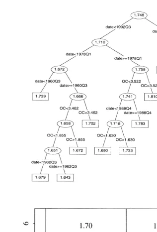
Another way of endogenously generating time-varying values of V*involves regression trees as described in Clark and Pregiborn (1991).5Application of the technique in our setup involves a binary recursive partitioning of the determinants of velocity, which we specify to be opportunity cost, OC, and time, TIME. In particular, if X is the space of OC and TIME over the sample, then the recursive algorithm partitions X into homogeneous rectangular regions x such that the conditional distribution of velocity given x does not depend on the specific values of OC and TIME, i.e., the tree is a step function that takes on a constant value of velocity within each region. One way of representing the results from this recursive algorithm is a tree (see Figure 3) with various nodes or branch points and terminal nodes, called leaves, placed at the end of the nodes.
In general, tree-based models can be interpreted as regressions on dummy variables, where the dummy variables are endogenously, recursively determined. They have several advantages: (a) they are invariant to monotone transformations of the independent vari-ables; (b) they are more adept at capturing non-additive behavior; (c) they allow more general interactions among independent variables. In particular, trees allow us to model relatively abrupt shifts in relationships, perhaps enabling us to track changes in
equilib-Figure 3. Regression tree for full data sample.
rium velocity non-parametrically. In addition, because the trees only depend on the ranks of the underlying data, in constructing our tree-based estimates, we do not need to take a stand on whether the relationship between velocity and opportunity costs is linear or logarithmic. To illustrate these concepts, Figure 3 displays two panels that represent alternatives ways of viewing the empirical estimates of a regression tree in which the GDP velocity of M2, V2, is the dependent variable and the variables,OC and TIME, are the independent variables, based on data from the entire sample from 1959:2 to 1997:4. The upper panel of Figure 3 shows the tree structure of the estimates; the full tree is an 11-way partition of the data, that is, it has 11 different terminal values of velocity depending on time and opportunity costs.6The top node, called the root, is designated by an oval; the average value of velocity for the whole period (1.748) is listed inside the oval. As we move down the tree the values of OC and TIME are successively split into finer branches, as indicated on the paths between nodes of the tree. For example, the top node splits on the left going down the tree on the basis of TIME for two splits until it splits on the right depending on whether OC is greater or less than 3.46. Rectangular boxes represent the 11 terminal nodes or leaves in this tree.
The lower panel of Figure 3 represents much of the same information as in the upper panel but in a way that highlights the time series structure of the relationship.7 For example, in the first six periods of the sample period, the value of the regression tree is 1.74, that is, the value of the GDP velocity of M2 is fixed at this value and does not depend on the level of opportunity costs. Thereafter, however, the level of the opportunity cost does matter with a three-way split (three values of velocity depending on the level of opportunity costs (OC) until the late 1980s, and a two-way split since then). As estimated, the tree provides a time-varying relationship between opportunity costs and velocity in which abrupt changes can occur.
The estimated regression tree does not necessarily give us a V*concept directly, except in the first six periods, because the summary measure of velocity in most of the terminal nodes depends on the level of opportunity costs. There are two alternative ways to proceed to fashion an estimate of V*from such a tree. We could prune the tree back to have a smaller number of splits or branches, and hope that the number of time periods in which
6We used the S-PLUS system to implement the tree-based regression models. The default algorithm
implemented there tends to estimate an “overly large tree’ with roughly N/10 terminal nodes, where N is the sample size. In our application where N5155, the number of nodes in the full model over the full period is 11. Such a size is in accord with the ”best current practice“ according to Clark and Pregiborn (1991, p. 415). However, as we shall see below, pruning the tree back (even severely) to have a smaller number of terminal nodes, appears to have very little effect on the estimates of V*relevant for our inflation forecast.
7These 11 rectangles represent contours of a step function that has a constant velocity value within each
rectangular region in the OCùTIME space and is zero elsewhere. In a regression tree with a dependent variable
that takes on numerical values as in our application using V2, the underlying statistical model posits that each observation, say yi, is distributed as normal with meanmiand constant variance where the step function being
determined by the regression tree can be thought of as the structural component,mi5vi(xi). The regression
surface in a regression tree consists of a linear combination of such step functions,vi(xi). Specifically, the overall
tree surface for a tree with p leaves ism~x! 5 (ip51miI$x [ Ni% 5 (ip51vi~xi!, where I is an indicator function
and the Niare disjoint hyper-rectangles with sides parallel to the coordinate axes. The deviance function is
defined to be D(mi; yi)5(yi2mi)2. At a given node, the mean parametermis constant for all observations. The
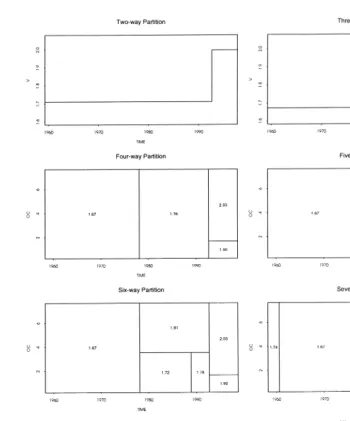
velocity does not depend on opportunity costs increases. For example, Figure 4 shows eight alternative partitions of the tree ranging from two to nine.8When the number of partitions is small, as in the upper portion of Figure 3, the periods in which velocity is independent of the level of opportunity costs are more numerous. For example, there is only one period at the end of the sample shown when velocity depends on opportunity
8Note that the companion to the panels in Figure 4 is the lower panel of Figure 3 that displays the full 11-way
partition of the tree. Figure 4. Tree partitions.
costs for the four-way partition and none for the two- and three-way partitions, shown in the top panel of the figure. Alternatively, when the partitions depend on the opportunity cost, in each quarter we could select the value corresponding to the historical average of the opportunity cost as our estimate of V*.
The two-way partition gives us a representation of V*as having a constant value a little over 1.7 until the early 1990s when it jumps to 2.0. The three-way partition adds an earlier step in 1978. Because the tree regression does not have the capability of directly representing a linear time trend, the presence of such a trend in the velocity data would be captured by splitting velocity in the middle of the full sample period, which is what our estimates do in the sample midpoint of 1978. Most notable, at least given our interest in forecasting inflation in the 1990s, is that the right-most part of the tree, which corresponds to this more recent period, remains invariant to the number of partitions that are used. Thus, our V*estimates do not appear to depend on the number of leaves in the tree, that is, the results hold under both parsimonious and profligate tree parameterizations.
Estimation
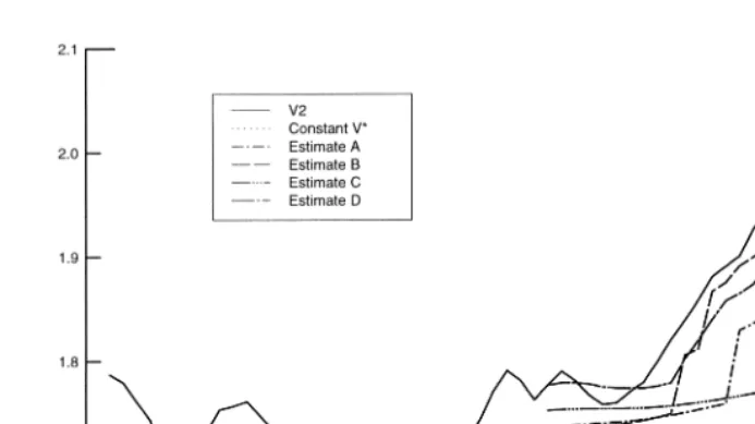
In Figure 5, we provide estimates of V* obtained from recursive estimation using the techniques described above. As indicated there, we are interested in determining how the various estimates of V*evolve in real time as they are supplied more observations, so we will update the estimates quarterly as each new observation becomes available.9The four alternative time-varying estimates shown with dashed and dotted lines correspond to the cases of a constant with one intercept shift, (Estimate A); a constant, constant trend and one intercept shift (Estimate B); the simplest regression tree specification with just two
9These calculations are only exercises in one sense: We do not deal explicitly with the fact that in real time
many of our data sources are preliminary. See Orphanides (1997) for a discussion of the problems associated with data revisions for the monetary policy process.
splits (Estimate C) and the full regression tree evaluated at the average opportunity cost, (Estimate D).
Three things are noteworthy here. First, even at the beginning of 1990, (when we first consider the additional flexibility in the specification of V*than the constant estimate) the point estimate of equilibrium velocity for the quarters shown appears somewhat higher than the constant V*estimate. This result is not surprising because, as already mentioned, a slight upward trend would appear to provide a better characterization of V*during the 1960 –1988 period over which the constant V*is computed. Second, and most important, compared with the fixed V* estimate, all four alternative recursive estimates show a dramatic upward shift in equilibrium velocity during the 1992–1994 period. The exact time at which this change is most noticeable differs quite significantly across the four estimates, with estimate B indicating a major shift as early as 1992, D in 1993, and estimate C detecting a large change only in late 1994. Third, despite the important timing differences in these estimates during 1992–94, it appears that by the end of the sample the four alternative estimates are in substantial agreement with one another.
Overall, while it would be difficult to judge the relative merits of these estimates of V* with such a short sample, the recursive estimates should be noted more for their similarity relative to the constant V*estimates, instead of their differences. The next step, then, is to use these estimates to construct the implied time series for P* and associated inflation forecasts.
III. Inflation Forecasts
Using the alternative concepts of V*shown in Figure 5, we next turn our attention to the inflation forecasts corresponding to the implicit alternative estimates of P*. We concen-trate on the simplest specification of the inflation equation in Hallman et al. that can provide 1-year-ahead forecasts of inflation (their equation 14):
D4p
t5a~pt212p*t21!1ut (6)
Hereptdenotes inflation over the four quarters starting with quarter t,D4is 4-quarter
difference operator, and p and p*denote the natural logarithms of P and P*, respectively.10 Using their data covering the period from 1955 to 1988, Hallman et al. estimatedato be
20:22 with a standard error of 0.044.11 Because of changes in the definitions of the variables and sample coverage, however, we need to reestimate this equation. Ending the sample in 1988 for comparability, we use overlapping quarterly data from 1960:1 to 1988:4. The revised estimate ofais20:16 with a standard error of 0.041 (obtained using the asymptotic correction for the moving-average error term).12
Figure 6 shows the in-sample inflation forecasts obtained from this equation as well as the out-of-sample forecasts based on the assumption of constancy for equilibrium velocity. As can be seen, while the forecast appears to move closely with realized inflation for most
10The dependent variable is the year-over-year change in the four-quarter change in the log of the price level.
That is,D4p
t5pt2pt245(pt132pt21)2(pt212pt25)5pt1322pt211pt25.
11The annual model in Hallman et al. uses only non-overlapping fourth quarter observations on inflation and
the price gap. Since we are interested in detecting changes in V*in real time, we adopt a setup that allows us
to use all quarterly observations.
12That is, because we are using overlapping, year-over-year inflation rates as the dependent variable in the
regression, the proper estimation of the asymptotic variance ofaneeds to take the error structure induced by using overlapping observations into account.
of the sample, since about 1992 forecasted inflation diverges from actual inflation with the forecast error becoming progressively worse until about 1995. The pattern of errors suggests that over this periodawas constructed using an estimate of equilibrium velocity that was likely systematically smaller than it should have been. This assessment is in agreement with the estimated upward shifting V* implied by the relationship between velocity and opportunity costs.
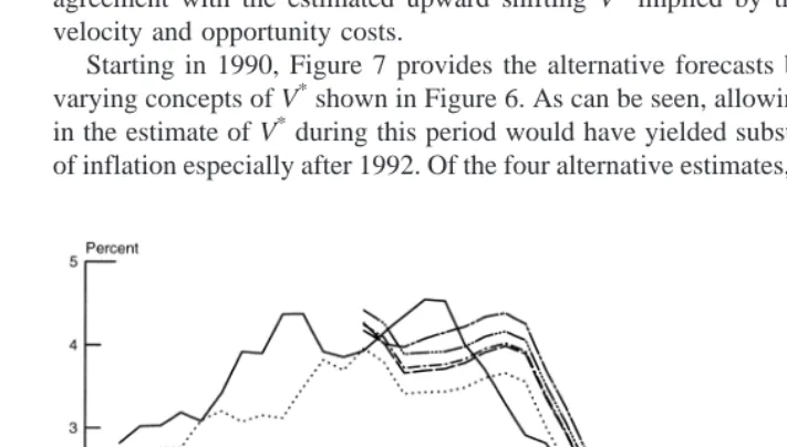
Starting in 1990, Figure 7 provides the alternative forecasts based on the four time-varying concepts of V*shown in Figure 6. As can be seen, allowing for the time variation in the estimate of V*during this period would have yielded substantially better forecasts of inflation especially after 1992. Of the four alternative estimates, it appears that Estimate
Figure 6. Inflation forecast assuming fixed equilibrium velocity.
B (obtained by estimating a one-time shift in V*and allowing for a time trend) and Estimate D (obtained from the full regression tree) would have resulted in the smallest forecast errors during this period. As shown in Table 1 for these two forecasts, the mean error was one-quarter of a percent or less and the mean absolute error was about half a percent. Indeed, this performance is better than the in-sample performance of the constant V*specification over the earlier period as shown in the memo item in the table.
Finally, the simplicity of the formulation we are examining allows us to easily characterize the specification error arising from incorrectly assuming a constant V* specification error arising from incorrectly assuming a constant V*specification when the correct specification should account for a one-time shift in velocity. If there were a one-time shift in equilibrium velocity from IE 5 here to IE 6 here, then the associated forecast error in forecasting inflation using the original estimate, IE 7 here, would be
2a~log~V2 *!
2log~V1 *!!
(7) Because the estimateda5 20.16 and the shift in V*appears to be from about 1.7 to 2, the implied inflation forecast error is about two and a half percent per 4-quarter period. Indeed, as shown in Figure 8, this is consistent with the magnitude of the recent forecast errors corresponding to the forecast obtained from the constant V*specification.
Alternative Non-Structural Approaches
The P*framework depends on only two parameters, V*the equilibrium velocity, anda, the coefficient indicating what fraction of the lagged gap between the log of the price level and the log of P*is expected to close over the next four quarters. The forecasting results suggest that of these two parameters, the behavior of only one has been problematical, namely V*. By relaxing the assumption that this parameter is constant but leaving the other parameter fixed we were able to restore the accuracy of the model. The specification analysis presented at the end of the previous section suggests that a trial-and-error process could also lead to the eventual discovery that setting V* 52 would have corrected the forecasting problems of P*framework.
This result raises the question how well a simpler approach that updates V*based on the recent inflation error—without using the additional information contained in the opportunity cost of holding M2, that we brought to bear on the problem—would have
Table 1. Summary Error Statistics from Inflation Forecasts_a/
Statistic Constant Time Varying V* Estimates Memo Item:
V* A B C D
Constant V* 1961:1–1989;4
Mean Error 1.65 0.44 0.22 0.54 0.03 0.15
Standard 1.14 0.61 0.47 0.84 0.59 1.05
Deviation of Error
Mean Absolute Error 1.74 0.66 0.44 0.81 0.46 0.78
_a/ The 28 out-of-sample forecast errors (1991:1 to 1997:4) are defined as inflation over the four quarters ending with quarter t minus the forecast for the corresponding period, measured in percent. Constant V* is estimated as the mean of M2 over the period from 1960:1 to 1988:4; Estimate A allows for a one-time shift in the intercept; Estimate B allows for a time trend and a one-time shift in the intercept; Estimate C allows for a two-branch regression tree; Estimate D allows for a full regression tree evaluated at the average opportunity cost of holding M2.
performed. As is evident from Figures 5 and 6, such an approach would have created wildly divergent estimates of V*. In particular, estimates of V*would have tended to fall in 1991–1992 before eventually moving upward later. A less extreme non-structural approach lets us evaluate the importance of opportunity costs to our forecasting results. Suppose as an alternative to Estimates A and B we dropped the term in opportunity costs, OC, from the regressions but computed everything else in Estimates A and B as above. As would be expected, this method would also eventually pick up the upward movement in the equilibrium velocity. However, the recognition is delayed (by at least 1 year), resulting in a marked deterioration in the forecast accuracy of this alternative.
IV. Conclusions
Our paper lays out a structural strategy for constructing real-time estimates of V*. We demonstrate that with the appropriate adjustments to V*, the forecasting of the P*model is maintained. This demonstration of the reliability of the P*approach in the face of fairly massive changes in the financial service industry that occurred over this period is significant. Because it came about by simply incorporating information from a standard money demand specification to update the estimate of equilibrium velocity, it suggests that the simple dynamic version of the quantity equation represented by our revised P* approach is well worth having in the monetary practitioners’ toolkit.
The opinions expressed are those of the authors and do not necessarily reflect the views of the Board of Governors of the Federal Reserve System. We wish to thank John Carlson, John Duca, Jim Lee, Robert Rasche, and an anonymous referee for comments on earlier versions of this paper.
Data Appendix
potential output, Q*we rely on the estimates made by the Congressional Budget Office. (The Economic and Budget Outlook, United States Government Printing Office, 1998.)
References
Clark, L. A., and Pregiborn, D. 1991. Tree-based models. In Statistical Models in S (J. M. Chambers and T. J. Hastie, eds.). Pacific Grove, California: Wadsworth and Brooks.
Feinman, J., and Porter, R. D. September 1992. The continuing weakness in M2. Federal Reserve Board, Finance and Economics Discussion Series, No. 209.
Hallman, J., Porter, R. D., and Small, D. H. September 1991. Is the price level tied to the M2 monetary aggregate in the long- run? American Economic Review 81(4):841–858.
Ha¨rdle, W. 1990. Applied Nonparametric Regression. Cambridge: Cambridge University Press. Koenig, E. F. September 1994. The P* model of inflation, revisited. Federal Reserve Bank of Dallas,
Working Paper No. 94-14.
Moore, G. R., Porter, R. D., and Small, D. H. 1990. Modeling the disaggregated demands for M2 and M1: The U.S. experience in the 1980s. In Financial Sectors in Open Economies: Empirical
Analysis and Policy Issues (Peter Hooper et al., eds.). Washington, D.C.: Board of Governors of
the Federal Reserve System.
Orphanides, A. December 1997. Monetary policy rules based on real-time data. Finance and Economics Discussion Series, 9803.
Orphanides, A., Reid, B., and Small, D. H. November/December 1994. The empirical properties of a monetary aggregate that adds bond and stock funds to M2. The Federal Reserve Bank of St
Louis Review 76(6):31–51.
Whitesell, W. C., and Collins, S. February 1996. A minor redefinition of M2. Federal Reserve Board, Finance and Economics Discussion Series, 96-7.