www.elsevier.com/locate/eja
Modelling irrigation scheduling to analyse water management
at farm level, during water shortages
F. Labbe´
a
, P. Ruelle
a,
*, P. Garin
a
, P. Leroy
b
aCemgref – French Institute of Agricultural and Environmental Research, Irrigation Division, BP 5095, 34033 Montpelier Cedex, France
bINRA ESR, 78850 Grignon, France
Accepted 3 September 1999
Abstract
The area under irrigated corn has significantly increased in the Charente river basin during the last 10 years. Corn water requirements are maximum in the summer, the period with low water flows and highest environmental vulnerability. Periods of water shortage during which irrigation is temporarily forbidden occur frequently. To reduce water demand, specific water saving policies are required. This paper investigates irrigation management strategies at farm level during water shortages. A computer programme called IRMA is used to represent the farmer’s decision making process. The model was calibrated and validated using information collected through a detailed monitoring of irrigation and farming practices of three representative farms during two irrigation seasons. The accuracy of the model was good; the difference between measured and simulated cumulative water volume used was slightly less than 8.5%. Analysis of daily simulated water demand shows that farmers have adopted different strategies to deal with water shortages, depending on the physical and socio-economic characteristics of their farms. The application presented in this paper stresses the potential of the proposed approach, if used on a larger farm sample, to compare the expected impact of different water management policies on water demand and irrigation practices at the farm level. © 2000 Elsevier Science B.V. All rights reserved.
Keywords:Corn; Farm level; France; Irrigation scheduling; Modelling; Water demand
1. Introduction 105×106m3 of water drawn annually in the
Charente District1, the irrigation sector consumes
the bulk of the 60 Mm3 consumed during the
In the Charente river basin, located in the
central–western part of France, a total area of period of low water flow and competes severely
with the other sectors, such as domestic and indu-8500 ha is irrigated with water drawn from the
river and corn is grown in 90%of this area. Most strial water use and leisure, as well as affecting
aquatic life in the river. of the 275 irrigated farms get water from small
pumping stations which feed one to three farms In one year out of five, the total volume
avail-able for the irrigation season is below the each. Irrigation is on demand. Out of the
2000 m3/ha required to meet 85%of crop needs at maximum evapotranspiration (MET ). During
* Corresponding author. Tel.:+33-46704-6340;
water shortages, irrigation is partially restricted.
fax:+33-46763-5795.
E-mail address:[email protected]
1De´partement de la Charente. (P. Ruelle)
Pumping is temporarily forbidden, from one to level of decision covers implementation choices, defined as the sequence of actions taken to imple-seven days per week, depending on river flow
levels. The days of the week when irrigation is ment the strategy and to achieve production
objectives. forbidden also vary according to the location along
the river in order to spread the demand for water $ A production strategy is defined by: (i) the
overall production objectives (for instance to between water users as evenly as possible.
The construction of a new reservoir on the achieve a certain yield while minimising risk);
(ii) the acquisition of know-how and the choice Charente river is under way. However, the total
water demand will still exceed the total available of areas of specialisation (decisions related to
crop specialisation); and (iii) the decisions resource stored by this dam and short periods of
water shortage are still likely to occur during the which affect the structural characteristics of the
farm (investment decisions). irrigation season. As no additional dams will be
built and as new resources cannot be developed, $ The implementation tactic is the translation of
the production strategy into sub-objectives, the water crisis can only be solved by reducing the
demand for irrigation during the summer, through decision rules and indicators for action (Girard
et al., 1994). The implementation tactic defines water saving policies, such as water pricing or
quota systems. The impact of such policies on how the production system will be managed
during one cropping season, taking into account cropping pattern and seasonal water use has
already been analysed using micro-economic the variability of the environment (climate,
water resource availability). models (Montginoul et al., 1997). However, the
seasonal time-step used in these models is too large In this paper, we focus on the representation of
farmers’ implementation tactics. The model pre-to assess the impact of these policies on the daily
organisation of irrigation events and the effective sented below attempts to represent the sequence
of decisions taken by farmers during one cropping demand for water during shortage periods.
This paper presents a new approach which can season to implement the strategic choice and to
achieve their production objectives. be used to estimate the temporal distribution of
the demand for irrigation water within the season Farmers’ implementation tactics rely upon a
simplified representation of the complex system and which assesses the impact of specific water
saving policies on this demand. The approach is they operate.
$ Farmers have a provisional schedule that
based on a day to day analysis and modelling of
farmers’ irrigation decisions and practices. The divides the year intofinalised periodsand defines
the sequence of operations to be conducted results were obtained for three selected farmers
facing irrigation restrictions. The characteristics of during each of these periods (e.g. a water turn
between irrigated fields). the water demand assessed are compared with a
more classical soil–water balance approach, $ Just as time is divided into finalised periods,
space is divided into areas with specific pro-applied at the field level to estimate irrigation
water requirements. duction objectives (i.e. irrigation management
units, for example).
$ In addition, farmers have a set ofadaptive rules that are used on a daily basis, depending on 2. Methodology
farm indicators. An acceptable degree of flexi-bility is kept for unpredictable events (climate,
2.1. General concepts
resource shortage, breakdowns, etc.). This flex-ibility is translated into a set of rules for daily In this approach, we assume that farmers’
deci-sions related to irrigation result from two levels of irrigation decision making (Re´au, 1993; Balas
and Deumier, 1993; Leroy and Jacquin, 1994). decision. The first level concerns choice of strategy,
which consists of long and medium term decisions The management logic is based on synchrony
diachrony (rules for choosing between technical 2.2. Structure of the model
sequences) (Sebillotte and Soler, 1988; Papy,
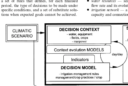
1994). Studies on farm implementation tactics The model consists of three components (Fig. 1):
(I ) thedecision contextwhich describes farm charac-have led to the concept of theaction model,
especi-ally on pressurised irrigation management teristics; (II ) thedecision modelwhich consists of a
set of rules; and (III ) the simulator engine which (Bonnefoy et al., 1992; Deumier and Peyremorte,
1993; Leroy et al., 1996; Lamacq et al., 1996; reproduces the decision sequence of the farmer. The
model takes as input climatic scenario and gives as Lamacq, 1997). This model was developed around
the following three points: output an irrigation schedule for all the plots of the
farm. The irrigation schedule is used by an
agro-$ one or several general objectives that define the
final goal towards which farmers’ decisions con- economic sub-modelto assess the yields and margins
obtained. The model is specified for each farm. This verge (for example, to achieve a target yield on
irrigated crops); model is implemented using the IRMA software
developed by Leroy et al. (1996).
$ a provisional schedule that set key moments
when the farm status is assessed and compared The variables describing thedecision contextare
based upon medium and long term farmers’ deci-with intermediate objectives, using specific
indi-cators (for example, vegetative state or soil sions, concerning conditions required to achieve
general objectives: condition);
$ a set of rules that defines, for each finalised $ water resources — seasonal irrigation volume,
flow rate and its evolution through the season; period, the type of decisions to be made under
specific conditions, and a set of substitute solu- $ irrigation network — a succession of pipes, their
capacity and connections to water resources; tions when expected goals cannot be achieved.
$ irrigation equipment — type, flow rate, time (often 7 and sometimes 10 days in the cases studied ).
needed to move it;
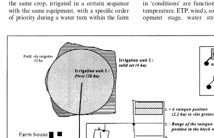
$ labour— number of available hours per day; $ Fields are divided into irrigation positions depending on the type of watering equipment $ fields — area, soil, seasonal cropping pattern
(crop and planting date), type and number of used (sets of irrigation sprinklers watering
simultaneously, lane spacing for a movable rain-irrigation sets;
$ irrigation blocks — bundling fields depending gun, sectors watered by a central pivot, etc.). Fig. 2 presents an example of a sample farm which on a given flow availability influenced by water
delivery constraints within the farm (water consists of two blocks, divided into several
irriga-tion units. resource, equipment).
Thedecision modelconsists of all therulesused by (ii) Rules for starting irrigation are described per crop. These rules are applied separately for the farmer to implement irrigation, which can be
classified into four categories. each irrigation management unit. They are either
recursive [AS LONG AS (condition 1 is true), IF (i) Rules to define irrigation units, in order to
simplify irrigation scheduling, for a given irrigation (condition 2 is true) THEN (irrigate)], or simulta-neous [AS SOON AS (condition 1 is true) THEN campaign.
$ Irrigation blocks are shared between irrigation (irrigate)]. Irrigation is defined either as an applied
depth or as an irrigation duration. Indicators used
management units, i.e. aggregating fields with
the same crop, irrigated in a certain sequence in ‘conditions’ are functions of climate (rainfall,
temperature, ETP, wind ), soil (ASW ), crop (devel-with the same equipment, (devel-with a specific order
of priority during a water turn within the farm opment stage, water stress), water resource
(volume already used, volume remaining), and AET and MET during the sensitive period of water stress derived from Doorebos and calendar (irrigation frequency, date).
(iii) Rules to split the season into finalised Kassam (1987), with local calibration.
The water demand estimated with the IRMA
periods. Rules for changing from one period to the
next are functions of calendar dates, or the first model is then compared with demand assessed by
a soil and water balance model used at field level irrigation of a given irrigation unit. For each
period, the sequence in which irrigation manage- (The PILOTE model ) developed by Mailhol et al.
(1997). This model is based on LAI simulation ment units are irrigated is described as well as the
rule in the case of rainfall and labour availability. and considers three separate storage capacities
along the soil profile, but does not take into Sequence defines priorities between fields.
(iv) Rules in case of rainfall are described, i.e. account farm strategies and implementation con-straints. It has been calibrated for corn (unpub-the amount of rainfall required to stop an
irriga-tion session, and the number of days for which lished data).
irrigation is postponed.
The simulator engine uses the variables of the decision context and the rules of the decision
model to mimic the farmer’s decision making 3. Construction of the model
process concerning irrigation. A timetable is
com-puted for each watering machine with a time step 3.1. Data collection
of 15 min. The irrigation schedule is given per day.
Taking this irrigation schedule as an input, the Using information collected through a
prelimi-nary survey of 30 farmers (10%sample), five distinct
agronomic sub-model assesses some indicators
related to the crop status and the expected yield types of farmer with different irrigation strategies
were identified. They are characterised in Table 1. for every field. It is a classic water balance model
coupled to a crop yield function. All the farms grow corn, but the importance of
other crops and livestock activities varies from one
$ The soil is viewed as a reservoir characterised
by a maximum available water storage farm to another. The main factors that explain the
different types of irrigation practice are the land
(MAWS ). MET is estimated from crop coeffi
-cientkdepending on development stages of the holding size and its ratio to the irrigated area,
irrigation equipment, economic dependency on irri-crop and reference Penman evaporation ( ET ).
$ Actual evapotranspiration (AET ) is parame- gated crops and farmer’s educational level
(Chazalon, 1995). Based on this analysis, samples terised by the empirical function of Baier
(1969). This relates AET to MET depending of three farms in 1996 and seven in 1997 were
selected to monitor irrigation practices during the on the actual soil water content in the reservoir.
When it becomes lower than an AET threshold whole irrigation campaign. The cases of three of
them with contrasting characteristics are presented value, it is reduced beneath MET. Drainage
estimation is based on the filling of the reservoir, here: a diversified cereal grower (G1), an intensive corn grower (G2), and a cattle breeder for whom in relation to MAWS but without upward
move-ment caused by capillary rise. irrigation remains a secondary activity (G4).
Detailed interviews on irrigation scheduling at
$ The simulation of the development stages of
the crop is obtained from threshold values of the tactical level have been undertaken for each
farmer to build their action model. More specifi-thermal time ( TT ) calculated from cumulative
mean daily temperature over a base temperature cally, the interviews were based on:
$ a field map, to define the irrigation management
as in Sepaskhah and Ilampour (1995). The yield is estimated by a relative yield, Y/Y
m, ratio of units according to the availability of water andlabour resources, the irrigation equipment, and respectively obtained yield and maximum yield
for a crop conducted at MET. It is a linear the type of crops;
$ a calendar to define the predefined schedule of
Table 1
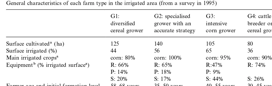
General characteristics of each farm type in the irrigated area (from a survey in 1995)
G1: G2: specialised G3: G4: cattle G5:
diversified grower with an intensive breeder or small diversified cereal grower accurate strategy corn grower cereal grower vine grower
Surface cultivateda(ha) 125 140 105 80 75
Surface irrigated (%) 44 56 65 36 34
Main irrigated cropsa corn: 80% corn: 100% corn: 95% corn: 90% corn: 92% Equipmentb(%irrigated surfacea) R: 66% R: 65% R:47% R: 74% R: 80%
P: 14% P: 18% P: 9% P: 14%
S: 20% S: 17% S: 44% S: 26% S: 6%
Farmer age and initial formation level 58–68 years, 35–50 years, 40–55 years, 30–45 years, 25–55 years, low medium/high medium/low medium/low medium
Number of irrigation units 2–3 3 3–4 1–2 1
Economic impact of irrigated crop medium high high medium/low low aMean value of the surface for the class.
bR, travelling raingun; P, central pivot; S, solid set.
field activities and irrigation events for each the average situation (see Table 2). The climatic
context in 1996 was rather dry, and irrigation management unit;
$ questions related to the possible strategies used started in mid-June. On the other hand, 1997 was
a rather wet year, and the rains in June postponed in terms of irrigation practices when confronted
with unpredictable events (rain, wind ) or irriga- the beginning of the irrigation season to mid-July.
In 1996, the arid conditions led to very low flows tion bans.
During the first season, information on the irriga- in the river and compulsory irrigation bans: two
days per week from mid-June to the beginning of tion calendar and volumes supplied by the
pump-ing station was collected for each irrigation unit. July, three days per week in July, and finally five
days per week in August. In 1997, the high rainfall, This information was compared with the
prelimi-nary output of the IRMA model constructed with late start of the irrigation season and releases from
the dam limited the irrigation bans to one day per the set of irrigation rules specified by the farmer
during the interviews. Additional rules were added week (normal conditions for that time of year) till
the end of July, when the bans were extended to to account for the adaptation to climatic events
and irrigation banning periods. The three action two days per week.
models were calibrated for the season, using
meas-urements on irrigation position duration and water 3.2. Building the action model of sample farmers
supplies.
A second series of interviews was conducted Table 3 presents the decision context and the
main decision rules for each sample farmer. before the irrigation season in 1997, to identify
possible changes in the decision context (i.e. the Irrigated areas of the farms are spatially organised
into one or two blocks that are composed of one cropping pattern or irrigation equipment) that
would require a change in the action model devel- to three management units depending on the
irriga-tion equipment used and the water turn plan. oped with the 1996 information. Then, the calendar
of irrigation events and the volume consumed for $ An indicator is computed for each farmer to
estimate the level of irrigation constraint at the
the different management units were collected
during the 1997 irrigation season. This information farm. This indicator is equal to the lowest of
the following two ratios: the pump flow rate was used to validate the model.
The approach was used for two contrasting over the cultivated area, and the watering
Table 2
Climatic context, total depths from 1st April to 30th September
Rain (mm) Penman evaporation (mm)
1996 1997 Average (1986–1997) 1996 1997 Average (1986–1997)
259 438 379 686 695 640
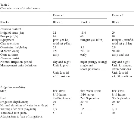
Table 3
Characteristics of studied cases
Farmer 1 Farmer 2 Farmer 3
Blocks Block 1 Block 2 Block 1 Block 1
Decision context
Irrigated area (ha) 32 15.4 29 40
Pumps (m3/h) 86 60 80 2×55
Equipment pivot (28 ha) raingun (60 m3/h) raingun (60 m3/h) raingun (2×40 m3/h) Characteristics solid set (4 ha) solid set (16 ha) solid set (3 ha)
Constraint (m3/h/ha) 2.8 3.9 2.9 2
MASWa(mm) 120 70–120 50–80 50–80
Corn earliness early early early and late early and late
Decision model
Normal irrigation period day and night night (energy saving) day and night day and night Management units definition Unit 1: pivot single unit: Unit 1: raingun; Unit 1: raingun;
seven positions seven positions eight positions Unit 2: solid Unit 2: solid Unit 2: raingun; set 1 position set; 10 positions eight positions
Unit 3: solid set; two positions
Irrigation scheduling
Start first stress first water stress first stress first stress 8/10 leaves 8/10 leaves 8/10 leaves 8/10 leaves
End 2nd September 2nd September 5th September 5th September
Irrigation depth (mm) 30 30–44 30–40 30
Normal duration of water turn (days) 7 7 7 7
Waiting after rain (day/mm) 1/5 1/5 1/10 1/7
Threshold rain (mm) 5 5 10 15
Adaptations to ban of irrigations:
2 days/week none none delay delay
3 days/week none watering night and delay delay
day
5 days/week delay watering night and missing out high delay in water turn day and delay MAWS fields
Strategy
Importance of irrigation middle, diversified low, mainly stock high, main activity
cereal grower breeder
Ratio: irrigated area/total area (%) 46 16 65
Objective corn yield (t/ha) 11.5 10 10
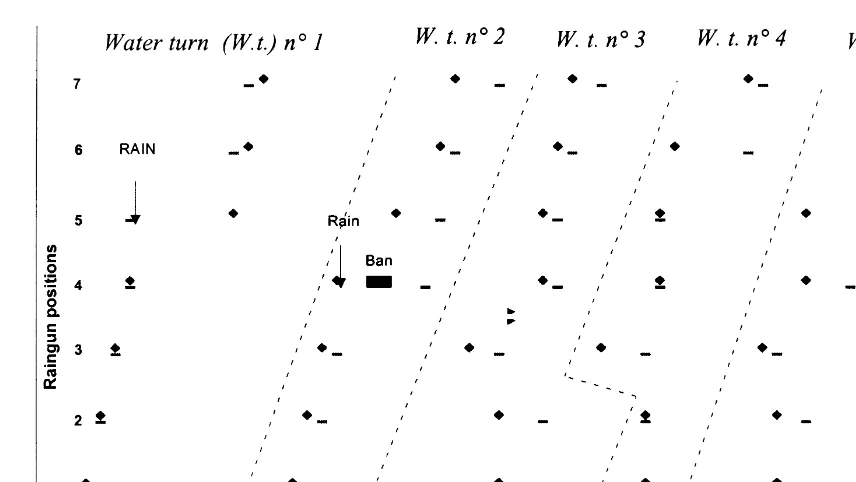
Fig. 3. Comparison of computed and measured irrigation calendars and water turns (Farmer 1, Block 2).
$ Farmer 1 has the highest value for this indicator, value of the indicator. The capacity of the
irrigation equipment and pumping station is i.e. 3.9 m3/h/ha for the block irrigated by a
raingun, and a lower value for the second block. limited and only sufficient for the organisation
of water turns during periods without shortage However, the second block is irrigated by fixed
irrigation equipment with greater flexibility and and bans. Also, the soil is rather shallow with
a poor retention capacity. Thus, the only avail-has the highest soil retention capacity. The
mean value for the whole farm is 3.2 m3/h/ha. able option to adapt to irrigation bans is to
delay water turns. As a result, satisfactory adaptability to the
rainfall and irrigation bans is obtained, that leads to high corn yields despite the fact that
corn cultivation is not the main activity of this 4. Results and discussion
sample farmer.
$ Despite adequate irrigation equipment, the indi- 4.1. Prediction of the irrigation calendar
cator is lower for Farmer 2, due to a limited
pumping capacity. With values of soil retention For the blocks irrigated either by a raingun or
by a solid set system, each water turn can be capacity between those of Farmer 1 and Farmer
3, and because of the secondary nature of defined by apositionor a sub-portion of the field
irrigated during the irrigation event which lasts irrigation on the farm, this farmer can afford
to forego irrigation sessions for some fields if from 8 to 10 h. For the central pivot of Farmer 1,
the irrigation calendar for any given location strict irrigation watering bans are in place. Also,
in the case of water shortage, low priority is within the field is defined as the dates the sprinklers
pass over this location. The predicted irrigation given to irrigation of areas under corn used
for silage. schedule was compared with the real irrigation
dates.
$ Farmer 3 has the most constraints from an
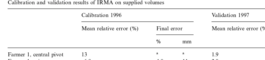
Table 4
Calibration and validation results of IRMA on supplied volumes
Calibration 1996 Validation 1997
Mean relative error (%) Final error Mean relative error (%) Final error
% mm % mm
Farmer 1, central pivot 13 a a 1.9 3.1 6
Farmer 1, raingun 6.8 4.8 11 3.8 5.4 13
Farmer 2 7.1 8 26 4.8 6.7 13
Farmer 3 6.8 8.5 2.6 3.6 5.4 8
aThe final measurement of this meter was not available.
predicted number of irrigation sessions is close throughout the entire season. For 1996, the
discrepancies remained below 7% for Farmer 2,
to the actual number of watering sessions.
$ The error between predicted and actual irriga- Farmer 3 and for the raingun block of Farmer 1.
The higher value for the central pivot of Farmer tion dates for thepositionsis one day on average
for rainguns and solid set systems. It is 1.5 days 1 (13%) is due to the high level of flexibility
afforded by the central pivot system already men-for the central pivot system, as this equipment
provides greater flexibility. tioned above, thus making the decision rules more
difficult to establish. For 1997, the errors are lower,
$ Some inaccuracies are due to unscheduled
deci-sions. For instance, on June 19, Farmer 1 has as a result of the lower water shortage and
reduc-tion in the number of irrigareduc-tion bans. The error irrigated two positions of Block 1 instead of
one. IRMA takes into account the rain of June in the total volume remains below 8.5% for 1996
and below 6.7% for 1997. Relating to the area
21 and delays the fifth position, whereas the
farmer delayed the sixth position (Fig. 3). irrigated and expressed in water depth (mm), the
errors are smaller than the depth provided by a
$ The gap between predicted and actual irrigation
dates does not increase over time, because farm- single irrigation position.
The simulation with the IRMA model provides ers repeatedly try to apply the predefined set of
rules that has been used to calibrate the model. an accurate aggregated demand for water on the
farm for the season. Also, it computes the water For example, Farmer 1 delays irrigation more
than expected after the July 1 rainfall and the demand for different time-steps. The accuracy of
the model remains very good for time-steps of the irrigation bans of July 3 and 4. However, the
gap between predicted and real dates is greatly same order of magnitude as the duration of a
water turn, but decreases as the time-step is reduced two weeks later ( Fig. 3).
shortened.
4.2. Prediction of supplied volumes
4.3. Assessment of pumping at daily time-steps in
Predicted volumes were compared with
mea-water shortage periods
sured volumes delivered to each farm by pumping stations. Table 4 presents the results of calibration
Because irrigation is banned on Sundays and validation with regard to volumes applied to
throughout the entire season, farmers spread their irrigated fields.
demand over the other days of the week. A reduc-The mean relative error2was used to assess the
tion in the number of days when irrigation is ability of the model to simulate volumes supplied
authorised is expected to lead to adaptations of the irrigation scheduling. The time-step considered
2Average of absolute values of (measured volume−simulated
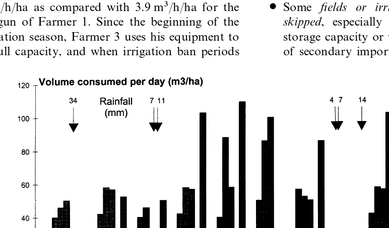
effect of irrigation bans on the demand for irriga- occur, he cannot increase watering time during authorised days of irrigation. The only alternative tion water.
Fig. 4 presents the daily water demand of the available to deal with the restrictions is to delay
water turns. As a result, the daily water draw raingun block of Farmer 1 as predicted by the
IRMA model. Under normal conditions, i.e. up to demand of Farmer 3 presents a much lower
vari-ability over time than those modelled for Farmer a weekly two day irrigation ban, the farmer can
afford to rely on night irrigation only (water turns 1. Four kinds of scheduling adaptation can be
identified. T1 and T2), and is irrigating at half his potential
of 50 m3/ha/day. From July 7 onwards, irrigation $ The water turn is extended timewise, and the
irrigation of one or morepositions is delayed.
is banned three days per week. Although the
rainfall delays the adaptation of the irrigation This simple option is better suited to restrictions
of short duration and good soils. However, it schedule, irrigation is performed during three days
(July 15, July 19 and July 22) to keep a constant may be the only option available to the most
constrained farmers. duration of the water turns. To deal with the
irrigation bans, the farmer intensifies the use of $ Theequipment can be used more intensively, to
avoid delaying the irrigation schedule and his irrigation equipment to maintain the same
duration of water turns. As stressed in Fig. 4, T1, water stress.
$ Theirrigation depth can be reducedin all fields T2, T5 and T6 have an equivalent duration, while
T3 and T4 have a shorter duration as there was or for fields with deep soil. This adaptation is
rarely implemented as it requires some adjust-no rainfall during these periods.
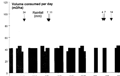
Similarly, Fig. 5 presents the demand for water ments of the irrigation equipment itself and
modification in the irrigation timetable. of Farmer 3, with an equipment constraint of
2 m3/h/ha as compared with 3.9 m3/h/ha for the $ Some fields or irrigation positions could be
skipped, especially for fields with good soil raingun of Farmer 1. Since the beginning of the
irrigation season, Farmer 3 uses his equipment to storage capacity or when the final corn yield is
of secondary importance because corn is used its full capacity, and when irrigation ban periods
Fig. 5. Impact of bans on daily demand (Farmer 3, Block 1, year 1996).
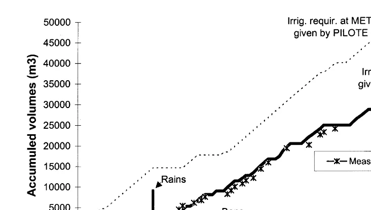
as silage (see Farmer 2). This adaptation is balance model PILOTE for the raingun block of
Farmer 1. Overall, the water balance model over-more likely to be implemented late in the season
once the period of highest stress sensitivity predicted by 42% the water demand for the entire
season. This overestimation is mainly due to an is over.
Lengthening the water turn, reducing the irrigation overprediction of the demand for irrigation events
early in the season, because irrigation equipment depth or skipping irrigation sessions for some
fields lead to water saving. However, increasing constraints were not considered. Once the
irriga-tion season has effectively started, the demand
the use of the irrigation equipment, the option
selected by Farmer 1, does not reduce the demand predicted by the two models follows the same
trend. In fact, farmers’ irrigation scheduling rules, for irrigation water. It only transfers the demand
to the authorised days. This kind of adaptation is specified in the IRMA model, do not consider
light falls of rain that reduce the crop water justified as the irrigation scheduling already based
on saving does not allow any reduction of supply requirements and that are accounted for in the
PILOTE model. However, this difference is levelled without causing water stress events. Systematic
overuse of equipment is then to be expected when out by higher irrigation depths predicted by the
IRMA model. From the end of July, as the fre-faced with temporary irrigation bans.
quency of irrigation bans increases, the gap between the cumulative demand predicted by the
4.4. Comparison between IRMA and PILOTE
two models increases again.
When PILOTE is run with the irrigation depth Fig. 6 compares the water demands defined by
the farmer and predicted with the IRMA model and calendar used by the farmer, it shows that
Fig. 6. Comparison of measured and predicted demand, Farmer 1, Block 1.
during another one in August (results not pre- The model was used to analyse the adaptation
of scheduling rules to water shortage situations or sented here). Corn yields obtained by the farmer
for the fields monitored range from 8.5 to 10.3 t/ha; temporary irrigation bans. Model simulations
stress the gap between the demand for water at values to be compared with the maximum yields
of 14 t/ha measured in experimental plots. As no the farm and theoretical crop water requirements.
The methodology developed provides an instru-other factor was limiting crop production, this
data confirms that crop water requirements have ment to compare different tools used in water
saving (bans, quotas, water pricing) which is com-not been fully met. In high demand periods, the
soil storage capacity remains at its critical thresh- plementary to the analysis undertaken with more
traditional micro-economic models. old, due to a late start of the irrigation campaign.
As a result, irrigation bans lead quickly to water The prospects for practical application of the
methodology are broad. The decision model cal-stress events with an expected negative impact on
crop yields. ibrated and validated enables, for example,
simula-tions under different climatic scenarios. The same decision model can be tested with 30 years of climatic data. As a given year is too marred by 5. Conclusions
climatic particularities to provide general results, several years of simulations would allow the The IRMA software that models the irrigation
decision making process allows accurate prediction stochastic dimension of the phenomenon to be
investigated. of the events of an irrigation season (dates and
volumes of water applied ) at the block or farm To address the issue of water shortage at the
scale of the Charente River Basin, a larger and scale. The average discrepancy between predicted
and observed irrigation dates is less than 1.5 day. representative sample of farmers should be selected
to represent the socio-economic and physical diver-The error in the cumulative volumes applied is
below 8.5% for the calibration year and 6.7% for sity within the basin. Using this representative
sample, a series of interviews and selected measure-the validation year; measure-the absolute value of error
concerning volumes is smaller than the water ments of water flows and demand would be
concernant le pilotage des irrigations. La Houille blanche
tative farm and to calibrate and validate the model.
2/3, 163–168.
Aggregated at the scale of the basin, the results of
Doorebos, J., Kassam, A.H., 1987. Re´ponses a` l’eau. Bull. FAO
the simulation for the various representative farms d’irrigation et de drainage 33 235 pp.
would provide a good estimate of the impact of Girard, N., Alain, H., Chatelin, M.-H., Gibon, A., Hubert, B., Rellier, J.-P., 1994. Formalisation des relations entre
stra-water saving measures. The results obtained should
te´gie et pilotage dans les syste`mes fourragers, Symposium
then be translated into simple recommendations
International Recherches — syste`mes en agriculture et
de´vel-for the management of dam releases and low
oppement rural, Montpellier, November, 223–228.
flow periods. Lamacq, S., Le Gal, P.Y., Bautista, E., Clemmens, A.J., 1996.
Farmers irrigation scheduling: a case study in Arizona, ASAE Proc. Int. Conf. on Evaporation and Irrigation Scheduling, San Antonio, TX, 3–6 November, 97–102. Lamacq, S., 1997. Coordination entre l’offre et la demande en
Acknowledgements eau sur un pe´rime`tre irrigue´: des sce´narios, des syste`mes et
des hommes. Ph.D. Thesis in Water Sciences. ENGREF,
The study behind this paper was carried out Montpellier, France, 137 pp.
Leroy, P., Jacquin, C., 1994. Un logiciel pour le choix de
l’as-with the financial support of the Conseil General
solement sur le pe´rime`tre irrigable d’une exploitation, 17th
de la Charente and is part of a global project on
European Regional Conference ICID, Varna, 16–22 May
the Charente River Basin, involving the various
Vol. 2., 61–72.
partners of water resources management. Leroy, P., Balas, B., Deumier, J.M., Jacquin, C., Plauborg, F.,
1996. Water management at farm level, Final Report 1991–1995 of EU CAMAR 8001-CT91-0109 Project: The Management of Limited Resources in Water and their Agroeconomical Consequences, 89–151., Chapter IV.
References Mailhol, J.-C., Olufayo, A., Ruelle, P., 1997. Sorghum and
sun-flower evapotranspiration and yield from simulated leaf area index. Agric. Water Manag. 35, 167–182.
Balas, B., Deumier, J.M., 1993. De l’entre´e parcellaire a` une
strate´gie globale de gestion de l’irrigation. Ame´nagements Montginoul, M., Rieu, T., Arrondeau, J.P., 1997. Une approche e´conomique pour concilier irrigation et environnement dans et Nature 14, 16–18.
Baier, W., 1969. Concepts of soil moisture availability and their le bassin versant de la Charente. ICID Workshop, 1977. Papy, F., 1994. Whole knowledge concerning technical system effect on soil moisture estimate from a meteorological
budget. Agr. Meteorol. 6, 165–178. and decision support. In: Dente, J.B., McGregor, A. ( Eds.), Rural Farming System Analysing. European Prospective. Bonnefoy, M., Bouthier, A., Deumier, J.-M., Jacquin, C.,
Leroy, P., 1992. E´ tude de faisabilite´ pour la mise au point CAB International, London, pp. 222–235.
Re´au, R., 1993. Exploitations de grande culture en Poitou-d’une me´thode de conduite des irrigations. ITCF-INRA.
39pp. Charente. Ame´nagements et Nature 111, 26–29.
Sebillotte, M., Soler, L.G., 1988. Le concept de mode`le ge´ne´ral Chazalon, J.M., 1995. La gestion de l’eau dans l’exploitation
agricole: e´tude comportementale cas des exploitations de et la compre´hension du comportement de l’agriculteur. C.R. Acad. Agric. Fr. 74 (4), 59–70.
grandes cultures du Nord Charente. DEA Socie´te´s
Ame´n-agement et De´veloppement Local, Universite´ de Pau et des Sepaskhah, A.R., Ilampour, S., 1995. Effect of soil moisture stress in evapotranspiration partitioning. Agric. Water Pays de l’Adour, 108 pp.