Vol. 43 (2000) 141–166
Optimal search on a technology landscape
Stuart Kauffman
a, José Lobo
b,1, William G. Macready
a,∗aBios Group LP, 317 Paseo de Peralta, Santa Fe, NM 87501, USA
bGraduate Field of Regional Science, Cornell University, 108 West Sibley Hall, Ithaca, NY 14853, USA
Received 16 September 1998; received in revised form 31 August 1999; accepted 12 October 2000
Abstract
We address the question of how a firm’s current location in the space of technological possi-bilities constrain its search for technological improvements. We formalize a quantitative notion of distance between technologies — encompassing the distinction between evolutionary changes (small distance) versus revolutionary change (large distance) — and introduce atechnology land-scapeinto an otherwise standard dynamic programming setting where the optimal strategy is to assign a reservation price to each possible technology. Technological search is modeled as move-ment, constrained by the cost of search, on a technology landscape. Simulations are presented on a stylized technology landscape while analytic results are derived using landscapes that are similar to Markov random fields. We find that early in the search for technological improvements, if the initial position is poor or average, it is optimal to search far away on the technology landscape; but as the firm succeeds in finding technological improvements it is optimal to confine search to a local region of the landscape. © 2000 Elsevier Science B.V. All rights reserved.
JEL classification:C61; C63; L20; O3
Keywords:Combinatorial optimization; Optimal search; Production recipes; Search distance; Technology landscape
1. Introduction
We address the question of how a firm’s current production practices and its location in the space of technological possibilities constrain its search for technological improvements. We formalize a quantitative notion of technological distance which encompasses the distinction
∗Corresponding author. Tel.:+1-505-992-6721.
E-mail addresses:[email protected] (S. Kauffman), [email protected] (J. Lobo), [email protected] (W.G. Macready).
1Tel.:
+1-607-255-5385.
between evolutionary change (small distance) versus revolutionary change (large distance). We are particularly interested in the relationship between the firm’s current location in the space of technological possibilities and thedistanceat which the firm should search for technological improvements. Our formalization results in aLandscape Search Model (LSM) search based upon atechnology landscapewhich extends traditional search theory. In the present discussion we focus on a detailed application of the LSM to optimal firm search.2 Sufficient detail is provided so that readers unfamiliar with the LSM will find a self-contained treatment.
The starting point for our discussion is the representation of technology first presented in Auerswald and Lobo (1996) and Auerswald et al. (2000). In this framework a firm’s production plan is more than a point in input–output space; it also includes theproduction recipeused in the process of production. Aconfigurationdenotes a specific assignment of states for every operation in the production recipe. A production recipe is comprised ofN distinctoperations, each of which can occupy one ofSdiscrete states. The productivity of labor employed by a firm is a summation over the labor efficiency associated with each of theNproduction operations. The labor efficiency of any given operation is dependent on the state that it occupies, as well as the states ofeother operations. The parametererepresents the magnitude of production externalities among theNoperations comprising a production recipe, what we refer to as “intranalities”. In the course of production during any given time period, the state of one or more operation is changed as a result either of spontaneous experimentation or strategic behavior. This change in the state of one or more operations of the firm’s production recipe alters the firm’s labor efficiency. The firm improves its labor efficiency — i.e., to say, the firm finds technological improvements — by searching over the space of possible configurations for its production recipe. When a firm finds a more efficient production recipe, it adopts that recipe in the next production period with certainty. In order to explicitly consider the ways in which the firm’s technological search is con-strained by the firm’s location in the search space, as well as the features of the space, we go beyond the standard search model (based on dynamic programming) and specify a technology landscape.Thedistance metricon the technology landscape is defined by the number of operations whose states need to be changed in order to turn one configuration into another. The firm’s search for more efficient, production recipes is studied here as a “walk” on atechnology landscape. Thecost of searchpaid by the firm when sampling a new configuration is a nondecreasing function of the number of operations in the newly sampled configuration whose states differ from those in the currently utilized production recipe.
The literature on technology management and organizational behavior emphasize that although firms employ a wide range of search strategies, firms tend to engage inlocal search — i.e., search that enables firms to build upon their established technology (see, e.g., Lee and Allen, 1982; Sahal, 1985; Tushman and Anderson, 1986; Boeker, 1989; Henderson and Clark, 1990; Shan, 1990; Barney, 1991; Helfat, 1994). As discussed in March (1991) and Stuart and Podolny (1996), the prevalence oflocal searchstems from the significant effort required for firms to achieve a certain level of technological competence, as well as from the greater risks and uncertainty faced by firms when they search for innovations far away from their current location in the space of technological possibilities. Using both numerical
and analytical results we relate the optimal search distance to the firm’s initial productivity, the cost of search, and the correlation structure of the technology landscape. As a preview of our main result, we find that early in the search for technological improvements, if the firm’s initial technological position is poor or average, it is optimal to search far away on the technology landscape. As the firm succeeds in finding technological improvements, however, it is indeed optimal to confine search to a local region of the technology landscape. We also obtain the familiar result that there are diminishing returns to search but without having to assume that the firm’s repeated draws from the space of possible technologies are independent and identically distributed.
The outline of the paper is as follows. Section 2.1 presents a simple model of firm-level technology; production recipes are introduced in Section 2.1, production “intranalities” are defined in Section 2.2, and firm-level technological change is discussed in Section 2.3. The material in these sections draws heavily from Auerswald and Lobo (1996) and Auerswald et al. (2000) and further details can be found there. Section 3 develops the notion of a technology landscape, which is defined in Section 3.1. The correlation structure of the technology landscape is introduced in Section 3.2 as an important characteristic defining the landscape. Section 4 treats the firm’s search for improved production recipes as movement on its technology landscape. The cost of this search is considered in Section 4.1. Section 4.2 then presents simulation results of search for theNetechnology landscape model defined in Section 2.2. We then go on to develop an analytically tractable model of technology landscapes in Section 5. We also describe in this section how a landscape can be represented by a probability distribution under an annealed approximation. Section 6 considers search under this formal model. The firm’s search problem is formally defined in Section 6.1 and the important role of reservation prices is considered in Section 6.2. Section 6.3 determines the reservation price which determines optimal search and results are presented in Section 6.4. We conclude in Section 7 with a summary of results and some suggestions for further work.
2. Technology
2.1. Production recipes
A recent body of work, both empirical and theoretical, emphasizes the importance of firm specific characteristics for explaining technological change (for empirical contributions to this literature, see, e.g., Dunne, 1988, 1989; Audretsch, 1991, 1994; Davis and Haltiwanger, 1992; Bailey et al., 1994; Dwyer, 1995; Dunne et al., 1996; for theoretical contributions, see, e.g., Jovanovic, 1982; Herriott et al., 1985; Hopenhayn, 1992; Kennedy, 1994; Ericson and Pakes, 1995). Our representation of firm-level technology incorporates this perspective. A firm using production recipeωand labor inputlt producesqt units of output during
time periodt,
qt =F[θt, lt]. (1)
firm’s labor productivity (i.e., how much output is produced by a fixed amount of labor). Firm-level output is thus an increasing function of organizational capital,θ. A firm’s level of organizational capital is a function of theproduction recipeutilized by the firm. The firm’s production recipe encompasses all of the deliberate organizational and technical practices which, when performed together, result in the production of a specific good. (Our concept of organizational capital is very similar to that found in Presscott and Visscher (1980) and Hall (1993).) We assume, however, that production recipes as we define them are not fully known even to the firms which use them, much less to outsiders looking in. In order to allow for a possibly high-level of heterogeneity among production recipes utilized by different firms, we posit the existence of a set of all possible production recipes,Ω. We will refer to a single elementωi ∈Ω as a production recipe. The efficiency mapping
θ:ωi ∈Ω →R++ (2)
associates each production recipe with a unique labor efficiency.
Production recipes are assumed to involve a number of distinct and well-defined oper-ations. Denote byN the number of operations in the firm’s production recipe, which is determined by engineering considerations. Theith recipeωican then be represented by
ωi = {ω1i, . . . , ω j i, . . . , ω
N
i }, (3)
whereωji is the description of operationjforj =1, . . . , N. We assume that the operations comprising a production recipe can be characterized by a set ofdiscretechoices. These discrete choices may represent either qualitative choices (e.g., whether to use a conveyor belt or a forklift for internal transport), quantitative choices (e.g., the setting of a knob on a machine), or a mixture of both. In particular we assume that
ωji ∈ {1, . . . , S} (4)
for each i ∈ {1, . . . , N} and where S is a positive integer. Each operation ωji of the production recipeωican thus occupy one ofSstates.
We denote a specific assignment of states to each operation in a production recipe as a configuration. Making the simplifying assumption that the number of possible states is the same for all operations that comprise a given production recipe, the number of all possible and distinct configurations for a given production recipe associated with a specific good is equal to
|Ω| =SN. (5)
New production processes are created by altering the states of the operations which comprise a production recipe. Technological change in this framework takes the form of finding production recipes which maximize labor efficiency per unit of output (i.e., technological progress is Harrod-neutral).
The contribution to overall labor efficiency made by thejth operation depends on the setting or state chosen for that operation,ωji, and possibly on the settings chosen for all other operations,ω−i j ≡ {ωi1, . . . , ωij−1, ωji+1, . . . , ωNi }. Hence the labor efficiency of the jth operation is in general a functionφijofωijandωi−j, so that we can write
We assume that theN distinct operations that comprise the production recipe contribute additively to the firm’s labor efficiency
θ (ωi)= and the other operations are in the states encoded by the vectorω−i j. In our cooperative setting, operations act not to maximize their own labor efficiency, but rather the aggregate labor productivity of the firm (i.e.,θ (ωi)).
2.2. Production intranalities
Working from the view that an important role of the firm is to “internalize” externalities (Coase, 1937; Williamson, 1985), we assume that in the typical case there are significant external economies and diseconomies among theN operations comprising a production recipe — i.e. to say, significant production and management externalities existwithinthe firm. These “intranalities” can be thought of as connections between the operations con-stituting the production recipe (Reiter and Sherman, 1962). To say that a connection exists between two operations is simply to say that the performance of the two operations affect each other (positively or negatively) either bilaterally or unidirectionally.
For a production recipeω∈Ω, we define theproduction intranalityscalar
ejk =e(ωk, ωj) (8)
as follows:
ejk= (
1, if the setting of operationjaffects the labor requirement of operationk,
0, otherwise (9)
forj, k=1, . . . , N. Since the choice of the setting for thejth operation always affects the efficiency for thejth operation, we haveejj =1 forj = 1, . . . , N. We make the strong simplifying assumption of equal number of connections, namely
ejk =ejk≡e. (10)
We assume throughout thateandN are given by nature. Whene=1, Eq. (8) is additively separable, otherwise
θ (ωi)=
2.3. Firm-level technological change
We now describe the general features of the technological problem facing the firm in our model. The firm’s production recipe determines the firm’s level of organizational capital and thus its labor efficiency. The production recipe is comprised of a number of distinct operations which at each moment can be in one of a finite number of possible, and discrete, states. Consequently, improvements in the technology used by the firm entails changes in the state of the operations comprising the production recipe.3 Firm-level technological
im-provements result from the firm finding improved configurations for its production recipe. Thus stated, the firm’s technological problem is a combinatorial optimization problem (Re-iter and Sherman, 1965; Papadimitriou and Steiglitz, 1982; Cameron, 1994). A compelling question to ask in the context of combinatorial optimization is, whether the globally optimal configuration can be reached from any given initial configuration.
We propose to study the firm’s technological problem by means of atechnology land-scape, developed in Section 3. The economies or diseconomies resulting from the interaction among the operations constituting the production recipe constraintgreatly affect the firm’s search for technological improvements. The intranalities parametereprovides a measure of the conflicting constraints confronting the firm as it seeks to optimize its production recipe. Just as a topographical map is a way of representing height over a two-dimensional physical space, a technology landscape is a means of representing the problem faced by the firm in its search for the optimal configuration for its production recipe.
3. The technology landscape
3.1. Defining the technology landscape
To define a technology landscape we require a measure of distance between two different production recipes,ωi andωj, each drawn fromΩ. The distance metric used here is not
based on the relative efficiencies of production recipes, but rather on the similarity between the operations constituting the recipes. More precisely, thedistanced(ωi, ωj)between the
production recipesωiandωjis theminimumnumber of operations which must be changed
in order to convertωitoωj. Since changing operations is symmetricd(ωi, ωj)=d(ωj, ωi).
Given this distance metric, we can define the set of “neighbors” for any production recipe,
Nd(ωi)= {ωj ∈ {Ω−ωi}:d(ωi, ωj)=d}, (12)
whereNd(ωi)denotes the set ofd-neighborsof recipeωi andd ∈ {0, . . . , N}.
With this definition of distance between recipes, it is straightforward to construct the technological graph,Γ (V , E). The set of nodes or vertices of the graph,V, are the pro-duction recipesωi ∈Ω. The set ofedgesof the technological graph,E, connect any given
3Our view of technological innovation is similar to that of Romer (1990), who remarks that over the past few
recipe to itsd =1neighbors, i.e., to the elements ofN1(ωi). For any production recipe,
the number of one-operation variant neighbors is given by
|N1(ωi)| =(S−1)N for all ωi ∈Ω. (13)
Thus each node ofΓ is connected to(S−1)Nother nodes.
The technology graph Γ and the efficiency map θ : Ω → R (efficiencies can be associated with each node in Γ) constitute a technology landscape. (For a comprehen-sive discussion of landscape models, see Stadler, 1995.) Assume, for the moment, that the labor efficienciesθ (ωi)are known with certainty for eachωi ∈Ω. Adopting some method
for tie-breaking, we can orient the edges of the graphΓ from vertices with higher labor effi-ciencies toward vertices associated with lower labor effieffi-ciencies. The firm’s search problem can then be recast as that of “moving” in the technology landscape (varying the production recipe by changing the state of at least one operation) in order to maximizeθ. The “steps” constituting such a walk represent the adoption, by the firm, of the sampled variants for its production recipe.
In the more general (and interesting) case where the efficiencyθ (ω)associated with each production recipe is not known with certainty, arandom field,F, can be defined over the production recipesω∈Ω by the joint probability distribution
F (θ1, . . . , θSN)=Prob{θ (ωi)≤θi fori=1, . . . , SN}, (14)
whereθ (ωi)∈Γ is the labor requirement at vertexi, eachθiis a positive scalar andSNis
the total number of vertices (i.e., of production recipes).4 The joint probability distribution in Eq. (14) induces a probability measure µon(θ1, . . . , θSN). The mapping implicit in
Eq. (2), along with the measureµ, forms a probability space which is a random field on Γ, the technological graph (see Macken and Stadler, 1995). In general then, a technology landscape is a realization ofF(Stadler and Happel, 1995).
3.2. Correlation structure of the technology landscape
Perhaps one of the most important properties of a technology landscape is itscorrelation structure. The correlation of a landscape measures the degree to which nearby locations on the landscape have similar labor efficiencies. A straightforward way to measure the correlation of a landscape is by means of the correlation function
ρ(d)= E(θ (ωi)θ (ωj)|d)−E(θ (ωi))E(θ (ωj)) σ (θ (ωi))σ (θ (ωj))
, (15)
whereσ (θ )is the standard deviation of efficiencies andρ(d)is the landscape’s correlation coefficient for efficiencies corresponding to production recipes ωi and ωj which are a
distanced apart (Eigen et al., 1989). The expectationE(θ (ωi)θ (ωj)|d)is with respect to
the probability distributionP (θ (ωi), θ (ωj)|d)which will be defined later in Section 5.
In the case of an Netechnology landscape the level of intranalities characterizing a production recipe induces thecorrelation structureon the landscape. To see this, consider
the limiting case of a production method characterized bye=1. In this case the contribu-tion made by each operacontribu-tion to overall produccontribu-tion cost is independent of the states of the other operations since the contribution to total efficiency made by each operation depends only on the state of that operation. Whether or not each operation in the production recipe makes its highest possible contribution to total efficiency depends in turn on whether or not the operation in question occupies its optimal state. Therefore, there exists a single glob-ally optimal configuration for the firm’s production method under which each operation occupies its optimal state. Any other configuration, which must necessarily have lower ef-ficiency, can be sequentially changed to the globally optimal configuration by successively changing the state of each operation. Furthermore, any such suboptimal recipe lies on a connected pathway via more efficient one-operation variants to the single global optimum in the landscape. Given the additive specification for production efficiency, a transition to a one-operation variant neighbor ofωi (i.e., changing the state of one operation) typically
alters the efficiency of the production method by an amountO(1/N ). Whene=1, pro-duction methods a distanced =1 away in the efficiency landscape therefore have nearly the same efficiency. Consequently, production methods in ane=1 landscape are tightly correlated in their production efficiencies.
In contrast, in thee=Nlimit the contribution made by each operation to the efficiency of the production method depends on the state of all other operations. The contribution made by each operation is changed when even a single operation is altered. Consider any initial pro-duction method among theSNpossible recipes. Alteration of one of the production method’s operations alters the combination of thee=Noperations that bear on the efficiency of each operation. In turn, this alteration changes the efficiency of each operation to a randomly chosen value from the appropriate distribution. The total production efficiency of the new production recipe is therefore a sum ofNnew random variables, from which it follows that the new efficiency is entirely uncorrelated with the old efficiency. The efficiency of any given production method is therefore uncorrelated with the efficiencies of its nearest neighbors.
Following Weinberger (1990) and Fontana et al. (1993), we can formally define a corre-lation coefficientfor anNelandscape. Suppose the firm moves from production methodωto production methodω′, a distancedapart. LetP (d)be the probability for any given operation to be among thedoperations that are changed by moving fromωtoω′. The autocorrelation coefficient,ρ(d), for two production methods a distancedapart is then given by
ρ(d)=1−P (d). (16)
The efficiency of an operation is unchanged if it is not one of thed operations that have been changed as the firm moved fromωtoω′, and if it is not one of theeneighbors of any of the changed operations. These two events are statistically independent, and thus
Whend =1 and there are no production externalities (e=1),ρ(1)≈1 for largeNand when every operation affects every other operation(e=N ), ρ(N )=0.
Ase increases, the landscape goes from being “smooth” and single peaked to being “rugged” and fully random. For low values ofethe correlation spans the entire config-uration space and the space is thus nonisotropic. Aseincreases, the configuration space breaks up into statistically equivalent regions, so the space as a whole becomes isotropic (Kauffman, 1993).
A related measure of landscape correlation, and one which can be used to compare landscapes, is thecorrelation length. The correlation length,l, of a technology landscape is defined by
l−1=X
d≥0
ρ(d). (19)
For a correlation coefficient which decays exponentially with distance, the correlation length is the distance over which the correlation falls to 1/eof its initial value. For theNetechnology landscape
l= − 1
lnρ. (20)
4. Search on the technology landscape
4.1. Search cost
The firm’s walk on a technology landscape is similar to a random search within a fixed population of possibilities (Stone, 1975).5 In the model presented here the firm seeks tech-nological improvements by samplingd-variants of its currently utilized production recipe. It does this by selecting independent drawings from some distributionF, at a sampling cost ofcper drawing (wherec >0). The firm’s search rule is fairly simple. Consider a firm that is currently utilizing production recipeωi and whose labor efficiency is thereforeθ (ωi).
The firm can take either of two actions: (1) keep using production recipeωi, or (2) bear an
additional search costcand sample a new production recipeωj ∈Ndfrom the technology
landscape. The decision rule followed by the firm is to change production recipes when an efficiency improvement is found, but otherwise keep the same recipe. Letθibe the efficiency
of the production recipe currently used by the firm, and letθjbe the efficiency of a newly
sampled production recipe; ifθj > θi, the firm adopts ωj ∈ Ω in the next time period;
ifθj ≤ θi, the firm keeps usingωi. This search rule is in effect an “uphill walk” on the
landscape, with each step taken by the firm taking it to ad-operation variant of the firm’s current production recipe.
The actual procedures used by the firm when searching for technological improvements can range from the non-intentional (e.g, “learning by doing”), to the strategic (investments
5Technological change has often been modeled by economists as a random search within a fixed population of
in R&D); technological improvements can result from small scale innovations occurring in the shop-floor or from discoveries originating in a laboratory. The level of sophistication of the firm’s search for new technologies is mapped into how many of the operations compris-ing the currently used production recipe have their states changed as the firm moves on its technology landscape. Production recipes sampled at large distances represent very differ-ent production processes while production processes separated by small distances represdiffer-ent similar processes. Improved variants found at large distances from the current recipe rep-resent wholesale changes whereas nearby improved variants constitute refinements rather than large scale alterations.
The many issues of industrial organizational, quality control, managerial intervention and allocation of scarce research resources involved in firm-level technological change are here collapsed into the cost,c, which the firm must pay in order to sample from the space of possible configurations for its production recipe. We assume the unit cost of sampling to be a nondecreasing function of how far away from its current production recipe the firm searches for an improved configuration — recalling that in the metric used here the distance between two configurations in the technology landscape is the number of operations which must be changed in order to turn one production recipe into the other. For present purposes it suffices to have the relationship between search cost and search distance to be a simple linear function of distances
c=αd, (21)
whereα∈ R+and 1 ≤d ≤ N is the distance between the currently utilized production recipe,ωi, and the newly sampled production recipe,ωj.
4.2. Search distance
At what distance away from its current production recipe should the firm search for technological improvements? In the most “naive” form of search on a technology landscape the firm restricts itself to myopically sampling among nearby variants in order to climb to a local optimum. Might it be better for the firm to search further away? The answer is “yes”, but the optimal search distance typically decreases as the labor efficiency of the firm’s current production recipe increases.
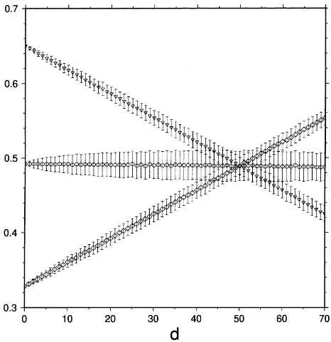
Fig. 1. Mean labor efficiencies±one standard deviation versus search distance forN =100, e=1, and three different initial efficiencies.
It thus seems plausible to suppose that, early in the firm’s search process from a poor or even average initial configuration, the more efficient variants will be found most readily by searching far away on the technology landscape. But as the labor efficiency increases, distant variants are likely to be nearly average in the space of possible efficiencies — hence less efficient — while nearby variants are likely to have efficiencies similar to that of the current, highly efficient, configuration. Thus, distant search will almost certainly fail to find more efficient variants, and search is better confined to the local region of the space.
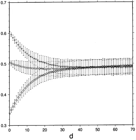
Fig. 2. Mean labor efficiencies±one standard deviation versus search distance forN =100, e=5, and three different initial efficiencies.
below the mean labor requirement found at that distance. Roughly one-sixth of a Gaussian distribution lies above one standard deviation. Thus, if six samples had been taken at each distance, and the “best” of the six chosen, then the expected increase in labor efficiency at each distance is represented by the envelope following the “plus” one standard deviation marks at each distance.
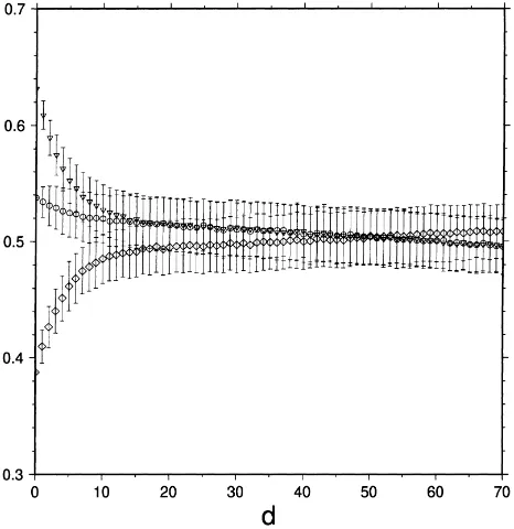
Fig. 1 shows that whene = 1 and the initial labor efficiency is near 0.5, the optimal search distance with six samples occurs when around 50 of the 100 operations are altered. When the initial labor efficiency is high, however, the optimal search distance dwindles to the immediate vicinity of the starting configuration. In contrast, when the initial labor efficiency is much lower than the mean, it is optimal for the firm to “jump” (i.e., search far away) instead of “walk” (i.e., search nearby) across the technology landscape. For Fig. 2, where e=5, the correlation length is shorter and as a result the optimal search distance for initial efficiencies near 0.5 is smaller (in this case aroundd =5). It is still the case that for highly efficient initial recipes, search should be confined to the immediate neighborhood. Very poor initial efficiencies still benefit most from distant search. In Fig. 3, wheree=11, the correlation length of the technology landscape is shorter still and optimal search distances shrink further.
Fig. 3. Mean labor efficiencies±one standard deviation versus search distance forN=100, e=11, and three different initial efficiencies.
It is appropriate to ask, however, how closely tied are the results to the adoption of a specific technology landscape model. In the next two sections we provide a framework with which to analytically consider the question of optimal search distance not just for anNelandscape but any landscape model. Section 5 outlines a formal framework with which to treat landscapes while Section 6 places search cost within a standard dynamic programming context.
5. Analytic approximation for the distribution of efficiencies
Technology landscapes are very complex entities, characterized by a neighborhood graph Γ and an exponential number of labor efficienciesSN. In any formal description of technol-ogy landscapes we have little hope of treating all of these details. Consequently we adopt a probabilistic approach focusing on the statistical regularities of the landscape and which is applicable to any landscape model.
and measuring on many landscapes then yields the desired aggregate statistics. Analytically mimicking this process is difficult, however, because averaging over the landscapes is the final step in the calculation and usually results in an intractable integration. In our annealed approximation the averaging over landscapes is donebeforemeasuring the desired statistic, resulting in vastly simpler calculations. The annealed approximation will be sufficiently accurate for our purposes and we shall comment on the range of its validity.
As an example of our annealed approximation, let us assume we want to measure the average of a product of four efficiencies along a connected walk inΓ. We label the effi-cienciesθ1,θ2,θ3, andθ4. IfP (θ1, . . . , θSN)is the probability distribution for an entire
technology landscape this average is calculated as
Z
θ1θ2θ3θ4P (θ1, . . . , θSN)dθ1· · ·dθSN
= Z
P (θ1, θ2, θ3, θ4) θ1θ2θ3θ4dθ1dθ2dθ3dθ4. (22)
This integral may be difficult to evaluate depending on the form ofP (θ1, θ2, θ3, θ4). Under the annealed approximation this integral is instead evaluated as
Z
P (θ1)θ1P (θ2|θ1)θ2P (θ3|θ2)θ3P (θ4|θ3)θ4dθ1dθ2dθ3dθ4, (23)
whereP (θ|θ′)is the probability that a configuration has labor efficiencyθconditioned on the fact that a neighboring configuration has efficiencyθ′.
As we have seen, under our annealed approximation the entire landscape is replaced by the joint probability distributionP (θ (ωi), θ (ωj)), where production recipesωiandωj are
a distance 1 apart inΓ. For any particular technology landscape the probability that the efficiencies of a randomly chosen pair of configurations a distancedapart have efficiencies θandθ′is
P (θ, θ′|d)= P
hωi,ωjidδ(θ −θ (ωi))δ(θ′−θ (ωj))
P
hωi,ωjid1
, (24)
where the notationhωi, ωjid requires that production recipesωi andωj are a distanced
apart andδ is the Dirac delta function.6 Rather than work with the fullP (θ, θ′|d) we simplify and consider only
P (θ (ωi), θ (ωj))≡P (θ (ωi), θ (ωj)|d=1). (25)
For some technology landscape properties we might need the fullP (θ (ωi), θ (ωj)|d)
dis-tribution but we will approximate it by building up fromP (θ (ωi), θ (ωj)). More accurate
extensions of this annealed approximation may be obtained ifP (θ (ωi), θ (ωj)|d)is known.
FromP (θ (ωi), θ (ωj))we can calculate bothP (θ (ωi)), the probability of a randomly
chosen production recipeωi having efficiencyθ (ωi), andP (θ (ωi)|θ (ωj)), the probability
6The Dirac delta function is the continuous analog of the Kronecker delta function:δ(x)is zero unlessx=0
and is defined so thatR
of a production recipeωihaving labor efficiencyθ (ωi)given that a neighboring production
recipeωj has labor efficiencyθ (ωj). Formally these probabilities are defined as
P (θ (ωi))=
Note that we have assumed, for mathematical convenience, that labor efficiencies range over the entire real line. While efficiencies are no longer bounded from below, the ordering rela-tionship amongst efficiencies is preserved and extreme labor efficiencies are very unlikely.
ForNelandscapes the following probability densities may be calculated exactly as:
P (θ (ωi))= loss of generality that the meanµ(θi)and varianceσ2(θi)of the technology landscape are
0 and 1, respectively. This annealed approach approximates theNetechnology landscape well whene/N ∼1, i.e., whenρ ∼0, but can deviate in some respects whene/N ∼0, i.e., whenρ ∼ 1 (see Macready, 1999). Eqs. (28)–(30) define a more general family of landscapes (sinceρcan be negative) characterized by arbitraryρ.
Since we are interested in the effects of search at arbitrary distancesdfrom a production recipeωi, we must inferP (θ (ωj)|θ (ωi), d)fromP (θ (ωi), θ (ωj)). We shall not supply this
calculation here but only sketch an outline of how to proceed (for full details, see Macready, 1999). To begin, note thatP (θ (ωj)|θ (ωi), d)is easily obtainable fromP (θ (ωi), θ (ωj)|d)as
ans-step random walk in the technology graphΓ beginning atωi and ending atωj has
labor efficienciesθ (ωi)andθ (ωj)at the endpoints of the walk. (Each step either increases
or decreases the distance from the starting point by 1.)P (θ (ωi), θ (ωj)|s)is straightforward
to calculate from Eq. (29).P (θ (ωi), θ (ωj)|d)is then obtained fromP (θ (ωi), θ (ωj)|s)by
including the probability that ans-step random walk onΓ results in a net displacement of d-steps. The result of this calculation is thatP (θ (ωj)|θ (ωi), d)is Gaussianly distributed
with a mean and variance given by
σ2(ωi, d)=1−ρ2d. (33)
Eqs. (32) and (33) play an important role in the next section.
6. Optimal search distance
6.1. The firm’s search problem
In order to determine the relationship between search cost and optimal search distance on a technology landscape, we recast the firm’s search problem into the familiar framework of dynamic programming (Bellman, 1957; Bertsekas, 1976; Sargent, 1987). Recall that each production recipeωi ∈ Ω is associated with a labor efficiencyθi. Production recipes at
different locations in the technology landscape — and therefore at different distances from each other — have different Gaussian distributions corresponding to differentµ(ωi, d)and
σ (ωi, d). The firm incurs a search cost,c(d), every time it samples a production recipe a
distancedaway from the current production recipe. The search costc(d)is a monotonically increasing function ofd since more distant production recipes require greater changes to the current recipe. For simplicity we takec(d)=αd(see Eq. (21)) but arbitrary functional forms forc(d)are no more difficult to incorporate within our framework. The firm’s problem is to determine the optimal search distance at which to sample the technology landscape for improved production recipes.7
To determine the optimal distance at which to search for new production recipes we begin by denoting the firm’s current labor efficiency byzand supposing that the firm is considering sampling at a distanced. IfFd(θ )is the cumulative probability distribution of
efficiencies at distanced, the firm’s expected labor efficiency,E(θ|d), searching at distance dis given by
E(θ|d)= −c(d)+β
z Z z
−∞
dFd(θ )+
Z ∞
z
θdFd(θ )
, (34)
whereβ is the discount factor. It may be the case that this discount factor isd-dependent since larger changes in the production recipe would likely require more time but we shall assume for simplicity thatβis independent ofd. The difference in labor efficiencies between searching at distancedand remaining with the current production recipe,Dd(z), is given by
Dd(z)=E(θ|d)−z= −c(d)−(1−β)z+β
Z ∞
z
(θ−z)dFd(θ ). (35)
Dd(z)is a monotonically decreasing function ofzwhich crosses zero atzc(d), determined
byDd(zc(d))=0. Forz < zc(d)it is best to sample a new production recipeωjsinceDd(z)
is positive. Ifz > zc(d)it is best to remain with the current recipeωibecauseDd(z)will be
negative and the cost will outweigh the potential gain. The zero-crossing valuezc(d)thus
7Note that sinceE[θ2]≪ ∞, by assumption, an optimal stopping rule exists for the firm’s search (DeGroot,
plays the role of the firm’sreservation price(Kohn and Shavell, 1974; Bikhchandani and Sharma, 1996). The reservation price at distancedis determined from the integral equation
c(d)+(1−β)zc(d)=β
Z ∞
zc(d)
(θ−zc(d))dFd(θ ). (36)
From Eq. (36) it can be seen that, as expected, reservation price decreases with greater search cost.
The firm’s optimal search strategy on its technology landscape can be characterized byPandora’s Rule: if a production recipe at some distance is to be sampled, it should be a production recipe at the distance with the highest reservation price. The firm should terminate search and remain with the current production recipe whenever the current labor efficiency is greater than the reservation price of all distances (a proof of this result is found in Weitzman, 1979).
6.2. The reservation price for Gaussian efficiencies
In the case where labor efficiencies at distanced are Gaussianly distributed, Eq. (36) reads as
(For clarity theddependence ofzchas been omitted.) Using the definite integral
Z ∞ function,8 we find that the equation determining the reservation price is
c(d)+(1−β)zc =β
To simplify the appearance of this equation we write it using the dimensionless variable
in terms of whichzc =
the equation which must be solved forδis therefore
A(ωi, d)=β
The explicitωi andd dependence ofAis obtained by plugging Eqs. (32) and (33) into
Eq. (44). Eq. (45) is the central equation determining the reservation pricezc(d).
Approxi-mate solutions to this equation are considered in Section 6.3. The optimal search distance,d∗, is now determined as
d∗=arg max
d
zc(d), (46)
where thed-dependence ofzc(d)is implicitly determined by Eq. (45). As a function ofd,
zcis well behaved with a single maximum so thatd∗is the integer nearest to thedwhich
solves∂dzc=0. We now proceed to find the equation whichd∗satisfies.
To begin, recall the definition ofδgiven in Eq. (41). Taking thed derivative ofδyields
∂dzc=
respectively, and we wish to express∂dδin terms of these known quantities. Differentiating
Eq. (45) with respect tod yields
∂dδ=
∂dA(ωi, d)
βerfc[−δ]−2 (50)
(assumingβis notd-dependent). Thusd∗is determined by
Using the definition ofAin Eq. (44) its derivative is easily found as
Plugging this result in Eq. (51) we find
0=√2 δ∂dσ+
which can be rearranged to give
0=2∂dc+
√
2(βδerfc[−δ]−2δ−A)∂dσ+β(erfc[−δ]−2)∂dµ. (54)
Finally, we use Eq. (45) to simplify this to
2
6.3. Determination of the reservation price
It is desirable to have an explicit solution forδ (implicitly determined by Eq. (45)). To this end we note some features of the function
DA(δ)≡β
A <0 then it is always profitable to try new production recipes. This is the case, e.g., when c(d)is negative and is sufficiently large in magnitude. We assume that the firm is not paid to try new production recipes and confine ourselves to the caseA >0.
In the caseA≫1, the solutionδofDA(δ)=0 is large and negative. In this case the term
multiplyingβis almost zero and to a very good approximation the solution ofDA(δ)=0
is
δ= −12A, (58)
orzc(d)= −c(d)+βµ(ωi, d). Thed dependence of the reservation price in this limit is
particularly simple
zc(d)=βθρd−αd. (59)
is too expensive or labor efficiencies are high and it is unlikely to find improved production recipes. We thus find that there are diminishing returns to search depending upon the firm’s current location in the technological landscape.
In the opposite limit, 0< A≪1, the solution is atδlarge and positive. In this case we use the asymptotic expansion9 smallAwe can use the asymptotic expansionW (x) ∼ lnx (see Corless et al., 1996) to write
In this section we present results for the optimal search distance as a function of: (i) the initial labor efficiency of the firm, (ii) the cost of search as represented byαinc(d)=αd; and (iii) the correlationρof the technology landscape. For brevity we will not present the βdependence but note thatβ <1 decreases the optimal search distance.
In appropriate parameter regimes we have used the approximations in Eqs. (58) and (61), elsewhere we have resorted to a numerical solution to Eqs. (45) and (55).
Figs. 4 and 5 present the optimal search distanced∗as a function of the firm’s current efficiency and the search cost parameter,α. In regions of parameter space in which the optimal search distance is zero it is best to terminate the search and not search for more
9TheΓfunction is defined byΓ (x)=R∞
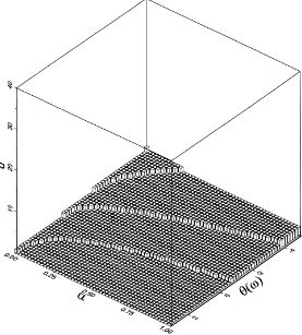
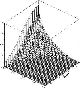
Fig. 4. Optimal search distanced∗as a function of the search costαand the initial labor efficiencyθ (ω)for a
landscape with correlation coefficient ofρ=0.3.
efficient production recipes. We note a number of features paralleling the simulation results presented in Section 4.2. In general, for low initial efficiencies it is better for the firm to search for improved production recipes farther away. As search costs increase (i.e., asα increases), the additional cost limits optimal search closer to the firm’s current production recipe. For production recipes which are initially efficient, the advantages of search are much less pronounced and for high enough initial efficiencies it is best to consider only single-operation variants. Again, a higher cost of search results in even smaller optimal search distances.
Fig. 5. Optimal search distanced∗as a function of the search costαand the initial labor efficiencyθ (ω)for a
landscape with correlation coefficient ofρ=0.9.
7. Conclusion
grounds the modeling of productive activity on engineering practice but unlike the early work attempts to provide a sufficient basis for modeling technological evolution.
In order to study how the current location of the firm in the space of technological possibilities affects the firm’s search for technological improvements, we model the firm’s search as movement on a “technology landscape”. The locations in the landscape correspond to different configurations for the firm’s production recipe. Local maxima and minima for the labor efficiency associated with each production recipe are represented by “peaks” and “valleys” in the landscape. The “ruggedness” of the landscape is in turn determined by the landscape’s correlation coefficient,ρ.
Our initial investigation about the firm’s optimal search distance involved computational exploration of theNetechnology landscape. The obtained simulation results prompted the development of a formal framework in which a technology landscape was incorporated into a standard dynamics programming model of search. The resulting framework abstracts away from all landscape detail except the important statistical structure which is captured in relatively simple probability distributions. As our main result we find that early in the search for technological improvements, if the initial position is poor or average, it is optimal to search far away on the technology landscape. As the firm succeeds in finding technological improvements, however, it is optimal to confine search to a local region of the technology landscape. Our modeling framework results in an intuitive and satisfying picture of optimal search as a function of the cost of search (which is itself a function of the distance between the firm’s currently utilized production recipe and the newly sampled recipe), the firm’s current location on the space of technological possibilities and the correlation structure of the technology landscape.
The general features of the story told in this paper — that early search can give rise to dramatic improvements via significant alterations found far away across the space of possi-bilities but that later search closer to home yields finer and finer twiddling with the details — suggests a possible application of our model to treat the development of “design types”. Among the stylized facts accepted by most engineers is the view that, soon after a major design innovation, improvement occurs by the emergence of dramatic alterations in the fundamental design. Later, as improvements continue to accumulate, variations settle down to minor fiddling with design details. We need only to think of the variety of forms of the early bicycles — big-front-wheel–small-back-wheel, small-front-wheel–big-back-wheel, various handle-bars — or of the forms of aircraft populating the skies in the early decades of the century.11
We believe that technology landscapes as introduced here can be a useful tool to study firm behavior. However, much future work clearly remains. Perhaps the most direct extension of our model would be to treat landscapes as Markov random fields where the full neighborhood N1around any particular configuration is included and results from the study of Markov random fields can be exploited (see, e.g., Kindermann and Snell, 1980). It would be desirable to build a model in which the correlationρof the technology landscape arises endogenously rather than treating it as an external parameter as we have done here.
11Dyson (1997) estimates that there were literally thousands of aircraft designs flown during the 1920s and 1930s
In this paper we have studied the optimal search distance for a single firm to sample its technology landscape. But as remarked by Stuart and Podolny (1996), firms do not search in isolation, rather they search as members of a population of simultaneously searching orga-nizations. How is the optimal search distance for an individual firm affected by the presence of other firms exploring the same technology landscape? If the cost of search increases with distance and optimal search distance decreases with increasing efficiency, how often will firms get “trapped” in suboptimal procedures or products? Since, in general, the structure of the technology landscape is only know locally, can a firm search in such a way so as to optimize both improvements on the landscape and learning about the landscape’s structure in order to guide further search? These and related questions await further investigation.
Acknowledgements
The authors thank Phil Auerswald, Richard Day, Richard Durrett, Alfred Nucci, Richard Schuler, Robert Solow, Nancy Stokey, Willard Zangwill and an anonymous referee for their helpful comments. The authors also gratefully acknowledge research support provided by the Santa Fe Institute and Bios Group LP.
References
Adams, J.D., Sveikauskas, L.,1993. Academic science, industrial R&D, and the growth of inputs. Center for Economic Studies Discussion Paper 93-1. US Bureau of the Census, Washington, DC.
Audretsch, D., 1991. New firm survival and the technological regime. Review of Economics and Statistics 73, 441–450.
Audretsch, D., 1994. Business survival and the decision to exit. Journal of Business Economics 1, 125–138. Auerswald, P., Lobo, J., 1996. Learning by doing, technological regimes and industry evolution. Presented at the
71st Annual Meeting of the Western Economic Association, San Francisco, CA.
Auerswald, P., Kauffman, S., Lobo, J., Shell, K., 2000. The production recipes approach to modeling technological innovation: an application to learning by doing. Journal of Economic Dynamics and Control 24, 389–450. Bailey, M.N., Bartelsman, E.J., Haltiwanger, J., 1994. Downsizing and productivity growth: myth or reality? Center
for Economic Studies Discussion paper 94-4. US Bureau of the Census, Washington, DC.
Barney, J.B., 1991. Firm resources and sustained competitive advantage. Journal of Management 17, 99–120. Bellman, R., 1957. Dynamic Programming. Princeton University Press, Princeton, NJ.
Bertsekas, D.P., 1976. Dynamic Programming and Stochastic Control. Academic Press, New York.
Bikhchandani, S., Sharma, S., 1996. Optimal search with learning. Journal of Economic Dynamics and Control 20, 333–359.
Boeker, W., 1989. Strategic change: the effects of founding and history. Academy of Management Journal 32, 489–515.
Cameron, P.J., 1994. Combinatorics: Topics, Techniques and Algorithms. Cambridge University Press, New York. Chenery, H.B., 1949. Engineering production functions. Quarterly Journal of Economics 63, 507–531. Coase, R., 1937. The nature of the firm. Economica 4, 386–405.
Cohen, W.M., Levinthal, D.A., 1989. Innovation and learning: the two faces of R&D. Economic Journal 99, 569–596.
Corless, R.M., Gonnet, G.H., Hare, D.E.G., Jeffrey, D.J., Knuth, D.E., 1996. On the LambertWfunction. Advances in Computational Mathematics 5, 329–359.
Davis, S.J., Haltiwanger, J., 1992. Gross job creation, gross job destruction, and employment reallocation. Quarterly Journal of Economics 107, 819–863.
Derrida, B., Pomeau, Y., 1986. Random networks of automata: a simple annealed approximation. Europhysics Letters 1, 45–49.
Dunne, T., Roberts, M., Samuelson, L., 1988. Patterns of firm entry and exit in US manufacturing industries. RAND Journal of Economics 19, 495–515.
Dunne, T., Roberts, M., Samuelson, L., 1989. The growth and failure of US manufacturing plants. Quarterly Journal of Economics 104, 671–698.
Dunne, T., Haltiwanger, J., Troske, K.R., 1996. Technology and jobs: secular change and cyclical dynamics. NBER Working Paper 5656. National Bureau of Economic Research, Cambridge, MA.
Dwyer, D.W., 1995. Technology locks, creative, destruction and non-convergence in productivity levels. Center for Economic Studies Discussion Paper 95-6. US Bureau of the Census, Washington, DC.
Dyson, F., 1997. Imagined Worlds: The Jerusalem–Harvard Lectures. Harvard University Press, Cambridge, MA. Eigen, M., McCaskill, J., Schuster, P., 1989. The molecular quasispecies. Advances in Chemical Physics 75,
149–263.
Ericson, R., Pakes, A., 1995. Markov — perfect industry dynamics: a framework for empirical work. Review of Economic Studies 62, 53–82.
Evenson, R.E., Kislev, Y., 1976. A stochastic model of applied research. Journal of Political Economy 84, 265–281. Fontana, W., Stadler, P.F., Bornberg-Bauer, E.G., Griesmacher, T., Hofacker, I.L., Tacker, M., Tarazona, P., Weinberger, E.D., Schuster, P., 1993. RNA folding and combinatory landscapes. Physical Review E 47, 2083–2099.
Griffeath, D., 1976. Introduction to random fields. In: Kemeny, J., Snell, J., Knapp, A. (Eds.), Denumerable Markov Chains. Springer, New York.
Hall, R.E., 1993. Labor demand, labor supply, and employment volatility. NBER Macroeconomics Annual 6, 17–47.
Helfat, C.E., 1994. Firm specificity and corporate applied R&D. Organization Science 5, 173–184.
Henderson, R.M., Clark, K.B., 1990. Architectural innovation: the reconfiguration of existing product technology and the failure of established firms. Administrative Science Quarterly 35, 9–31.
Herriott, S.R., Levinthal, D.A., March, J.G., 1985. Learning from experience in organizations. American Economic Review 75, 298–302.
Hey, J.D., 1982. Search for rules of search. Journal of Economic Behavior and Organization 3, 65–81. Hopenhayn, H., 1992. Exit, entry, and firm dynamics in long run equilibrium. Econometrica 60, 1127–1150. Jovanovic, B., 1982. Selection and the evolution of an industry. Econometrica 50, 659–670.
Jovanovic, B., Rob, R., 1990. Long waves and short waves: growth through intensive and extensive search. Econometrica 58, 1391–1409.
Kauffman, S., 1993. Origins of Order: Self-organization and Selection in Evolution. Oxford University Press, New York.
Kennedy, P.M., 1994. Information processing and organizational design. Journal of Economic Behavior and Organization 25, 37–51.
Kindermann, R., Snell, J.L., 1980. Markov Random Fields and their Applications. American Mathematical Society, Providence, RI.
Kohn, M., Shavell, S., 1974. The theory of search. Journal of Economic Theory 9, 93–123. Koopmans, T. (Ed.), 1951. Activity Analysis of Production and Allocation. Wiley, New York.
Lee, D.M., Allen, T.J., 1982. Integrating new technical staff: implications for acquiring new technology. Management Science 28, 1405–1420.
Leontief, W.L., 1953. Studies in the Structure of the American Economy: Theoretical and Empirical Explorations in Input–Output Analysis. Oxford University Press, New York.
Levinthal, D.A., March, J.G., 1981. A model of adaptive organizational search. Journal of Economic Behavior and Organization 2, 307–333.
Lobo, J., Macready, W.G., 1999. Landscapes: a natural extension of search theory. Santa Fe Institute Working Paper 99-05-037E. The Santa Fe Institute, Santa Fe, NM.
Macken, C.A., Stadler, P.F., 1995. Evolution on fitness landscapes. In: Nadel, L., Stein, D. (Eds.), 1993 Lectures in Complex Systems. Addison-Wesley, Reading, MA.
March, J.G., 1991. Exploration and exploitation in organizational learning. Organization Science 2, 71–87. Marengo, L., 1992. Coordination and organizational learning in the firm. Journal of Evolutionary Economics 2,
Marsden, J.R., Pingry, D., Whinston, D., 1974. Engineering foundations of production functions. Journal of Economic Theory 9, 124–140.
Muth, J.F., 1986. Search theory and the manufacturing progress function. Management Science 32, 948–962. Nelson, R.R., Winter, S.G., 1982. An Evolutionary Theory of Economic Change. Belknap Press, Cambridge, MA. Papadimitriou, C.H., Steiglitz, K., 1982. Combinatorial Optimization: Algorithms and Complexity. Prentice-Hall,
Englewood Cliffs, NJ.
Presscott, E., Visscher, M., 1980. Organization capital. Journal of Political Economy 88, 446–461.
Reiter, S., Sherman, G.R., 1962. Allocating indivisible resources affording external economies of diseconomies. International Economic Review 3, 108–135.
Reiter, S., Sherman, G.R., 1965. Discrete optimizing. SIAM Journal 13, 864–889.
Romer, P.M., 1990. Endogenous technological change. Journal of Political Economy 98, 71–102. Sahal, D., 1985. Technological guideposts and innovation avenues. Research Policy 14, 61–82. Sargent, T.J., 1987. Dynamic Macroeconomic Theory. Harvard University Press, Cambridge, MA.
Shan, W., 1990. An empirical analysis of organizatonal strategies by entrepreneurial high-technology firms. Strategic Management Journal 11, 129–139.
Smith, V.L., 1961. Investment and Production: A Study in the Theory of the Capital-using Enterprise. Harvard University Press, Cambridge, MA.
Stadler, P.F., 1995. Towards a theory of landscapes. Social Systems Research Institute Working Paper No. 9506. University of Wisconsin, Madison, WI.
Stadler, P.F., Happel, R., 1995. Random field models for fitness landscapes. Santa Fe Institute Working Paper 95-07-069. The Santa Fe Institute, Santa Fe, NM.
Stone, L.D., 1975. Theory of Optimal Search. Academic Press, New York.
Stuart, T.E., Podolny, J.M., 1996. Local search and the evolution of technological capabilities. Strategic Management Journal 17, 21–38.
Tesler, L.G., 1982. A theory of innovation and its effects. The Bell Journal of Economics 13, 69–92.
Tushman, M.L., Anderson, P., 1986. Technological discontinuities and organizational environments. Administrative Science Quarterly 14, 311–347.
Vanmarcke, E., 1983. Random Fields: Analysis and Synthesis. MIT Press, Cambridge, MA.
Weinberger, E.D., 1990. Correlated and uncorrelated fitness landscapes and how to tell the difference. Biological Cybernetics 63, 325–336.
Weitzman, M.L., 1979. Optimal search for the best alternative. Econometrica 47, 641–654.