*Tel.: 001-704-547-3242; fax: 001-704-547-3123.
E-mail address:[email protected] (M.J. Khouja)
Optimal ordering, discounting, and pricing in the single-period
problem
Moutaz J. Khouja*
Information&Operations Management Department, The Belk College of Business Administration, The University of North Carolina at Charlotte, Charlotte, NC 28223, USA
Received 22 October 1998; accepted 23 March 1999
Abstract
The single-period problem (SPP), also known as the newsboy or newsvendor problem, is to"nd the order quantity
which maximizes the expected pro"t in a single-period probabilistic demand framework. Previous extensions to the SPP include, in separate models, the simultaneous determination of the optimal price and quantity when demand is price-dependent, and the determination of the optimal order quantity when progressive discounts with preset prices are used to sell excess inventory. In this paper, we extend the SPP to the case in which demand is price-dependent and multiple discounts with prices under the control of the newsvendor are used to sell excess inventory. First, we develop two
algorithms for determining the optimal number of discounts under"xed discounting cost for a given order quantity and
realization of demand. Then, we identify the optimal order quantity before any demand is realized. We also analyze the joint determination of the order quantity and initial price. We illustrate the models and provide some insights using
numerical examples. ( 2000 Elsevier Science B.V. All rights reserved.
Keywords: Inventory management; Production management; Operations management
1. Introduction
The classical single-period problem (SPP) is to
"nd a product's order quantity which maximizes the expected pro"t in a probabilistic demand framework. The SPP model assumes that if any inventory remains at the end of the period, one discount is used to sell it or it is disposed of [1]. If the order quantity is smaller than the realized de-mand, the newsvendor, hereafter NV, forgoes some
pro"t. If the order quantity is larger than the realiz-ed demand, the NV losses some money because he/she has to discount the remaining inventory to a price below cost. The SPP is re#ective of many real-life situations and is often used to aid decision making in the fashion and sporting industries, both at the manufacturing and retail levels [2]. The SPP can also be used in managing capacity and evaluat-ing advanced bookevaluat-ing of orders in service indus-tries such as airlines, hotels, etc. [3].
Several researchers have suggested SPP exten-sions in which demand is price dependent [4}10]. Whitin [4] assumed that the expected demand is a function of price and using incremental analysis, derived the necessary optimality condition. He then
provided closed-form expressions for the optimal price, which is used to "nd the optimal order quantity for a demand with a rectangular distribu-tion. Mills [5] also assumed demand to be a ran-dom variable with an expected value that is decreasing in price and with constant variance. Mills derived the necessary optimality conditions and provided further analysis for the case of de-mand with rectangular distribution.
Lau and Lau (LL) [6] introduced a model in which the NV has the option of decreasing price in order to increase demand. LL analyzed two cases for demand:
(a) CaseA: Demand is given by a simple homo-scedastic regression model x"a!bP#e, where
aandbare constants,xis the quantity demanded,
P is unit price, andeis normally distributed. The above equation implies a normally distributed de-mand with an expected value which decreases lin-early with unit price.
(b) CaseB: Demand distribution is constructed using a combination of statistical data analysis and experts'subjective estimates. The &method of mo-ments'was used to"t the four-parameter beta dis-tribution to estimate demand.
For case A, LL showed that the expected pro"t is unimodal and thus the golden section method can be used for maximization. For case B, there is no guarantee the expected pro"t is unimodal. Thus, LL developed a search procedure for identifying local maximums. LL also solved the problem under the objective of maximizing the probability of achieving a target pro"t and considered both zero and positive shortage cost cases. For zero shortage cost and demand given by case A, LL derived closed-form solutions for the optimal order quanti-ty and optimal price. For zero shortage cost and demand given by case B, LL developed a procedure for computing the probability of achieving a target pro"t and used a search procedure for "nding a good solution. For positive shortage cost and demand given by cases A or B, the probability of achieving a target pro"t may not be unimodal. LL developed procedures for computing the probabil-ity of achieving a target pro"t and identifying a good solution.
Polatoglu [7] also considered the simultaneous pricing and procurement decisions. Polatoglu
identi"ed few special cases of the demand process addressed in the literature: (i) an additive model in which the demand at price P is x(P)"k(P)#e, where k(P) is the mean demand as a function of price, and e is a random variable with a known distribution and E[e]"0, (ii) a multiplicative model in whichx(P)"k(P)ewhereE[e]"1, (iii) a riskless model in which X(P)"k(P). Polatoglu analyzed the SPP under general demand uncertain-ty to reveal the fundamental properties of the model independent of the demand pattern. Polatoglu assumed an initial inventory of I,k(P) is a monotone decreasing function of P on (0,R), and a"xed ordering cost ofk. For linear expected demand, (k(P)"a!bP, where a,b'0) Polatoglu proved the unimodality of the expected pro"t for uniformly distributed additive demand and exponentially distributed multiplicative demand.
Khouja [8] solved an SPP in which multiple discounts are used to sell excess inventory. In this model, retailers progressively increase the discount until all excess inventory is sold. The product is initially o!ered at the regular priceP0. After some time, if any inventory remains the price is reduced to P
1,P0'P1. In general, the prices are
P
i,i"0, 1,2,n, wherePi'Pi`1. The amount
de-manded at each P
i is assumed to be a multiple t
i,i"1,2,nof the demand at the regular priceP0.
Khouja solved the problem under two objectives: (a) maximizing the expected pro"t, and (b) maxi-mizing the probability of achieving a target pro"t. Khouja showed that the expected pro"t is concave and derived the su$cient optimality condition for the order quantity. For maximizing the probability of achieving a target pro"t, Khouja provided closed-form expression for the optimal order quantity. Khouja [10] developed an algorithm for identifying the optimal order quantity for the multi-discount SPP when the supplier o!ers the NV an all-units quantity discount. Khouja and Mehrez [9] provided a solution algorithm to the multi-product multi-discount constrained SPP.
quantity exceeds the realized demand. Most retailers, for example, do not use a single discount to sell excess inventory as assumed in the classical SPP. The assumption of multiple discounts pro-posed by Khouja [8] contributes a step toward solving this problem. However, Khouja's model is limited in that it assumes that the discount prices are preset and are not part of the decisions of the NV. The model also assumes that the quantity sold at each discount price is a given multiple of the quantity sold at the initial price without any assumptions about demand}price relationship. Finally, the model assumes that discounting a product does not incur a "xed cost, whereas many retailers incur a "xed discounting cost resulting from the need to advertise the dis-count and markdown the disdis-counted items. In this paper, we extend the SPP to the case in which:
1. demand is price dependent,
2. multiple discount prices are used to sell excess inventory,
3. the discount prices used to sell excess inventory are under the control of the NV, and
4. there is a positive setup cost associated with discounting a product due to the costs of advert-ising and marking down the discounted items. The resulting problem is composed of two small-er problems. In the"rst problem, for a given realiz-ation of demand, a given demand}price relation-ship, and a given order quantity, the NV must determine the optimal discounting scheme. This problem will be referred to as the discounting prob-lem. In the second problem, the NV must determine the order quantity which maximizes the expected pro"t prior to any demand being realized. This problem will be referred to as the order quantity problem.
In the next section, we review the classical SSP. In Section 3, we analyze the discounting problem and develop two algorithms for determining the optimal discounting scheme under two di!erent assumptions about the behavior of the NV. In Section 4, we solve the optimal order quantity problem. In Section 5, we analyze the joint quantity
and initial pricing decisions. We conclude in Sec-tion 6.
2. Basic results and problem motivation
De"ne the following notation:
x "quantity demanded, a random variable,
f(x)"the probability density function ofx,
F(x)"the cumulative distribution function ofx,
P "per unit selling price,
C "per unit cost,
< "per unit salvage value,
S "per unit shortage penalty cost,
C
0 "C!<, per unit overage cost,
C
6 "P!C#S, per unit underage cost, and
Q "order quantity, a decision variable. The pro"t per period is
n"
G
(P!C)Q!S(x!Q) ifx*Q,Px#<(Q!x)!CQ ifx(Q. (1) Simplifying and taking the expected value ofngives the following expected pro"t:
E(n)"(P#S!C)
P
=Q
Qf(x) dx!S
P
= Qxf(x) dx
#(P!<)
P
Q 0xf(x) dx!(C!<)
P
Q 0Qf(x) dx. (2) Let the superscript H denote optimality. Using Leibniz's rule to obtain the"rst and second deriva-tives ofE(n) shows that it is concave, and thus, the su$cient optimality condition is to set the "rst derivative to zero which yields the well-known frac-tile formula:
F(QH)"P#S!C
P#S!<. (3)
Suppose the NV uses multiple discounts to sell excess inventory. In this case, the SPP decomposes into two problems: the discounting problem and the order quantity problem. The sequence of events in the SPP is as follows: (1) The NV sets the initial price at which to o!er the product (P
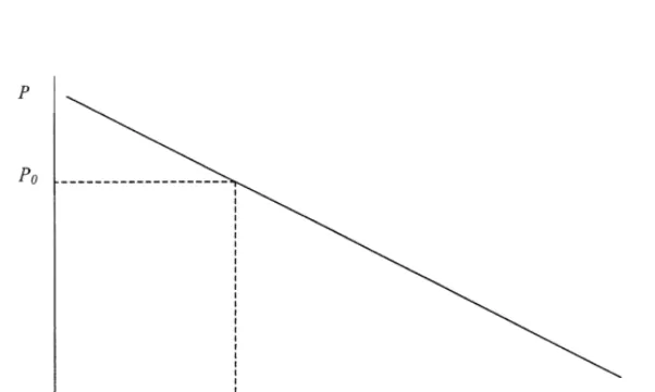
Fig. 1. Expected demand as a function of price. Table 1
Prices for di!erent discounting schemes on [0,P
0]
Number of prices,h Prices used,P i
1 P
0, 0
2 P
0,P0/2, 0
3 P
0, 2P0/3,P0/3, 0
4 P
0, 3P0/4,P0/2,P0/4, 0
2. 2.
h P
0, (h!1)P0/h, (h!2)P0/h,2,P0/h, 0
2. 2.
n P
0, (n!1)P0/n, (n!2)P0/n,2,P0/n, 0
competitive situation of the"rm, (2) The NV deter-mines the order quantity (Q), (3) The NV"nds out the quantity demanded at P
0, and (4) The NV
determines the discounting scheme to use. In order to determine the optimal order quantity, the discounting problem must be solved "rst. In ana-lyzing the discounting problem, we assume: 1. The relationship between demand and price is
linear and is given by
P"=!bx, (4)
wherebis a positive constant known to the NV from historical data and=is a random variable
with a known distribution but whose actual real-ization becomes known only after ordering. The demand function in Eq. (4) is the classical func-tion used in economics. This assumpfunc-tion implies that the NV knows how demand changes with price (i.e. demand elasticity), but does not know the initial level of demand (x
0) when the product
is o!ered at an initial price ofP
0(he/she knows
the expected value E(x
0)"k0). After the NV
ordersQunits and the selling period begins,x0, and thus =, become known. Fig. 1 shows the
expected demand as a function of price. 2. The discounts are equally spaced in terms of
price on the domain [0,P
0]. While this
assump-tion restricts the opassump-tions available to the NV, it
signi"cantly simpli"es the analysis and allows us to focus on the e!ects of progressive discounting on the SPP. Let
h"1,2,n, the number of prices to use to sell the
product (excluding 0), a decision variable,
P
i"theith selling price, and
F"the"xed cost of discounting which includes the cost of advertising and marking down the discounted items.
The prices charged under di!erent values ofhare as shown in Table 1. Note that for any h, the order quantity may not be large enough to o!er the product at lower prices. Let x
Fig. 2. Demand distribution when the item is o!ered at unit priceP
0.
Table 2
Prices for di!erent discounting schemes on [P a,P0]
Number of prices,h
Prices used,P i
2 P
0,Pa
3 P
0, (P0#Pa)/2,Pa
4 P
0, (2P0#Pa)/3, (P0#2Pa)/3,Pa
5 P
0, (3P0#Pa)/4, (P0#Pa)/2, (P0#3Pa)/4,Pa
2. 2.
h P
0, ((h!1)P0#Pa)/h, ((h!2)P0#2Pa)/h,2,
(P
0#(h!1)Pa)/h,Pa
2. 2.
n P
0, ((n!1)P0#Pa)/n, ((n!2)P0#2Pa)/n,2,
(P
0#(n!1)Pa)/n,Pa
demanded at an initial price ofP
0. From (4)
P
0"=!bx0. (5)
Since=is a random variable with a known
distri-bution,x
0is a linear function of a random variable
and is also a random variable with known distribu-tion. Fig. 2 shows the distribution ofx
0for
normal-ly distributed=.
The discounting scheme in Table 1 assumes that unit prices are set at equal intervals on the range [0,P
0]. On the other hand, the classical SPP
as-sumes that whatever remaining inventory can be sold at a price (i. e. salvage value) of<. LetP
abe the
price at which all of Q will be sold. Then, the assumption that all remaining inventory can be sold at a price of<implies that<)P
a. Therefore,
an alternative discounting range is [P
a,P0] with
prices as shown in Table 2.
We use the discount range of [0,P
0] because
it allows for the option of not discounting at
all which may be pro"table when there is a small quantity left and the"xed cost of discounting is large. In addition, any discounting scheme shown in Table 2 for a given value of h may be approximated using larger values ofhin Table 1. For example, whenP
a"<"P0/2, using four
pri-ces on the range [P
a,P0] may be approximated by
using six prices on the range [0,P
0] (of which the
last 3 will not be used since all inventory is sold prior to reaching those prices).
3. The discounting problem
The NV starts by o!ering the product at a price of P0, which we, for now, assume to be based on competitive considerations. The NV waits until sales start slowing down which indicates that demand at the current price is almost fully satis"ed. The NV then plan to discount the product soon. Therefore, the NV at this phase of the problem has perfect knowledge of demand (i.e. the realization of= or x
0is known). In this
sec-tion, we analyze the problem of deciding on the discount prices. The NV can follow one of two policies in discounting: A Blind policy, denoted by B, and a Revenue maximizing policy, denoted by M.
Blind policy(B): The NV keeps discounting the product until all inventory is sold or a price of zero is reached (i.e. items discarded). Note that the NV in this case is not concerned with whether the remaining inventory is worth discounting in terms of covering the "xed discounting cost. This policy can be justi"ed on the basis that the NV deals with a large number of products and does not have completely accurate and timely inventory records, which makes it easiest to keep discount-ing until all inventory is sold. For a given Q, the NV must determine the value ofhwhich maximizes revenue. Let P
a be the price at which all of Q
will be sold. Then, for example, if the NV o!ers the product at only one price (P0), the revenue is given by
R
B(h"1)"
G
P
0Q ifPa*P0
P
0x0 ifPa(P0.
R
B(h"4)"
G
P
0Q if Pa*P0,
P
0x0#(3P0/4)(Q!x0)!F if 3P0/4)Pa(P0,
P
0x0#(3P0/4)(P0/4b)#(P0/2)(Q!P0/4b!x0)!2F if 2P0/4)Pa(3P0/4,
P
0x0#(3P0/4)(P0/4b)#(P0/2)(P0/4b) #(P
0/4)(Q!P0/2b!x0)!3F if P0/4)Pa(2P0/4,
P0x0#(3P0/4)(P0/4b)#(P0/2)(P0/4b)
#(P
0/4)(P0/4b)!3F if Pa(P0/4.
Simplifying gives
R
B(h"4)"
G
P
0Q if Pa*P0,
(3P
0/4)Q#(P0/4)x0!F if 3P0/4)Pa(P0,
(2P
0/4)Q#(2/4)P0x0#P20/16b!2F if 2P0/4)Pa(3P0/4,
(P
0/4)Q#(3P0/4)x0#3P20/16b!3F if P0/4)Pa(2P0/4,
P
0x0#6P20/16b!3F if Pa(P0/4.
(7)
In general, for any number of pricesh, the revenue is given by
R
B"
G
P
0Q if Pa*P0,
j
hP0x0# h!j
h P0Q# P20
bh2
j~1
+ i/0
i!jF if h!j
h P0)Pa(
h!j#1
h P0, P
0x0#
P20
bh2
h~1
+ i/0
i!(h!1)F if P a(
P
0
h.
(8) If the NV o!ers the product at four prices
(P
0, 3P0/4, 2P0/4, andP0/4) then, using (5), the
incremental quantity demanded at each dis-count price is P
0/4b and the revenue is given
by
Obviously, ifP
a'P0(or equivalentlyQ(x0) then
no discounts are needed andhH"1. De"nekas
k"max
G
h:h!1h P0)Pa(P0
H
.In other words, k is the largest number of prices which satis"es [(k!1)/k]P
0)Pa. Lemmas 1 and
2 are introduced to develop an algorithm which can e$ciently identifyhH.
Lemma 1. The optimal number of prices at which to ower the product satisxeshH*k.
Proof. The proof of Lemma 1 is provided in the appendix.
Lemma 2. For any number of prices v such that
v'kand for any integer j, if
v!j
v P0)Pa(
v!j#1
v P0and
v#1!j
v#1 P0)Pa(
v!j#2
v#1 P0,
then the revenue from using h"v#1 is greater than or equal to the revenue from using h"v (i.e.
R
B(v#1)*RB(v)).
Proof. The proof of Lemma 2 is provided in the appendix.
Algorithm 1: Blind policy
Step 1: Compute P
a using (4). If Pa*P0 then
stop, all ofQwill be sold at the initial priceP
0.
Step 2: Find the largesthfor which [(h!1)/h]
P
Ifk"nthen stopkis optimal. (by Lemma 1) Seti"n
Step 3: Find the largest integer, j, for which [(i!j)/i]P
0)Pa([(i!j#1)/i]P0.
If [(i!j!1)/(i!1)]P
0)Pa([(i!j)/(i!1)]P0,
thenh"i!1 is suboptimal. (by Lemma 2)
Step 4: Set i"i!1. Ifi'k#1 go to Step 3.
Compute revenue using (8) for h"k and all
h'knot found to be suboptimal. Selecthwith the largest revenue.
Steps 1 and 2 are performed once. Step 2 requires more computations than Step 1 and is bounded by
n. In the worst case, Step 3 is performedntimes and each of these iterations is bounded by n. Finally, Step 4 is bounded byn. Therefore, the running time of the algorithm is O(n2).
Revenue maximizing policy (Policy M): Here, the last discount (j) for a given number of prices (h) is o!ered only if the additional revenue from it is greater than or equal to the"xed cost of discount-ing (F). Thus, if (h!j)P
0/h)Pa((h!j#1)P0/h
then discount j is used only if the additional rev-enue it generates from selling the additional units demanded between prices (h!j)P
0/handPa is
greater than or equal toF. To simplify the analysis, we introduce the following realistic assumption:
Assumption 1. The largest number of prices the NV may use (n), is such that the incremental revenue from selling all units demanded between prices 2P
0/nandP0/nis greater than F.
In other words, the NV will not use prices so close to each other to the point where the incremen-tal revenue of a discount is insu$cient to cover the
"xed cost of the discount. From (5) the quantities sold at 2P
0/n and P0/n are (=!P0/n)/b and
(=!2P
0/n)/b, respectively. Thus, the incremental
units sold atP"P
0/nareP0/nband the
incremen-tal revenue is (P
0/nb)P0/n"P20/bn2. Assumption
1 can be restated as
P20
bn2*F. (9)
In order to derive the revenue function under this policy, we need to introduce a new policy, denoted C. Suppose that discount j is not used unless the full quantity demanded at that discount price is available. When the quantity available at discountjis small, the"xed cost of discounting will be greater than the incremental revenue from sell-ing this small quantity. Thus, discountsell-ing will re-duce revenue and R
C'RB. When the quantity
available at discount jis large (but insu$cient to satisfy all of the incremental demand at that price), the"xed cost of discounting will be smaller than the incremental revenue from selling this large quanti-ty. Thus, discounting will increase revenue and
R
C(RB. To obtainRC, the revenue from the last
discount is eliminated from the expression for
R
Band the coe$cient of Fis reduced by one. For
example, the revenue functions forh"2 and 4 in policy C are:
R
C(h"2)"
G
P
0Q if Pa*P0,
P
0x0 if P0/2)Pa(P0,
P
0x0#P20/4b!F if Pa(P0/2.
(10)
and
R
C(h"4)"
G
P
0Q if Pa*P0,
P
0x0 if 3P0/4)Pa(P0,
P
0x0#3P20/16b!F if 2P0/4)Pa(3P0/4,
P
0x0#5P20/16b!2F if P0/4)Pa(2P0/4,
P
0x0#6P20/16b!3F if Pa(P0/4.
In general, for anyh,R
From (8) and (12), the di!erence in revenue between the Blind policy and policy C is
R
Mbe the revenue of the Revenue Maximizing
policy, (R
B!RC) will be used to"ndhwhich
maxi-mizes R
M. For a givenQ and h, if (RB!RC)'0
then the last discount should be used andR
M"RB.
If (R
B!RC)(0 then the last discount should not
be used andR
M"RC. Because under the Revenue
Maximizing policy the last discount may or may not be used we must"nd bothhHandjH. Note that
handhHare used to denote the number of prices and the optimal number of prices, respectively, for both the B and M policies. Using the de"nition of
kintroduced before Lemma 1, Lemma 3 introduces important properties ofRM.
Lemma 3. The optimal number of prices at which to ower the product satisxeshH*k or hH"1.
Proof.The proof of Lemma 3 is provided in the appendix.
Algorithm 2: Revenue maximizing policy
Step 1. Compute P
a using (4). If Pa*P0 then
stop, all ofQwill be sold at the initial priceP
0.
Step 3. Find the largest integer, j, for which [(h!j)/h]P
M(h) using the function constructed in
Steps 2 and 3 for allh*k.
Selecthwith the largest revenue.
R
M"
G
0.5P
0x0#0.5P0Q!F"$206,700 if h"2,
P
0x0#2P20/bh2!F"$208,089 if h"3,
2P
0x0/4#2P0Q/4#P02/bh2!2F"$208,400 if h"4,
2P
0x0/5#3P0Q/5#P02/bh2!2F"$209,000 if h"5,
3P
0x0/6#3P0Q/6#3P02/bh2!3F"$208,433 if h"6,
3P0x0/7#4P0Q/7#3P20/bh2!3F"$208,620 if h"7.
(14) is bounded byn. In the worst case, Step 3 is
per-formed n times and each of these iterations is bounded by n. Finally, Step 4 is bounded by n. Therefore, the running time of the algorithm is O(n2).
Numerical Example 1. Consider a product with demand functionP"=!0.01x, where=is
nor-mally distributed with a mean of 110 and a stan-dard deviation of 10. This implies an increase of 100 units in demand for each$1 drop in price. The"xed cost of discounting is F"$800. Suppose the NV ordered Q"10,750 units and is using the Blind
policy. The NV o!ered the product at an initial price ofP
0"$20 and found that the realization for = was 120 or equivalentlyx
0"10,000 units The
question facing the NV is how many prices to use to sell all ofQ? The NV limits the number of possible prices at which to o!er the product ton"7 which satis"es assumption 1. Thus, the choice ofhmust to be made fromh"1, 2,2, 7. Using (4), the price at
which all of the 10,750 units will be sold is
P
a"$12.5. Algorithm 1 shows that one of the
values of h"2, 5, or 7 is optimal. Using (8) with
Q"10,750 givesR
B(h"2)"$206,700,RB(h"5)"
$209,000, and R
B(h"7)"$208,620 and thus,
hH"5, which corresponds to discounts of 20% from the original price and unit prices of
$20.00, $16.00, $12.00, $8.00, and $4.00. The last unit in Q"10,750 will be sold for $12.00. If the value ofbis changed tob"0.02, which implies a 50 unit increase in demand for each $1 drop in unit price, and the realization of = is changed to ="220, then the realized demand at P
0"$20
remains x
0"10,000. However, the optimal
number of prices decreases to hH"4 with
R
B(h"4)"$205,100. Because the additional
quantity sold at each discount is smaller with the newb, then it is optimal to use smaller number of prices and larger discounts. If the value of F
is changed to F"$3,200 then it is optimal to use hH"2 for which R
B(h"2)"$204,300.
Because the cost of discounting is higher, it is opti-mal to use a sopti-maller number of prices and larger discounts.
Now suppose the NV is using a Revenue Maxi-mizing policy. The application of Algorithm 2 for
Q"10,750 andP
a"$12.50 results in the following
revenue function:
Thus, hH"5,jH"2,RHM"RHB"$209,000 and the Blind and the Revenue Maximizing policy give the same results. ForQ"10,680, P
a"$13.2
and the Blind policy gives hH"5, and
RHB"$208,160 whereas the Revenue Maximizing policy gives hH"6, jH"2, and RHM"$208,400 which corresponds to discounts of 16.67% from the initial price.
4. The order quantity problem
a givenhis We simplify (15) and "ndQH for normally and uniformly distributed demand.
4.1. Uniform demand distribution
Supposex
0is uniformly distributed on the range
[a,b], then Eq. (15) gives
Lemma 4.The expected proxt function is concave in Q for uniformly distributed demand.
Proof. The proof of Lemma 4 is provided in the appendix.
Thus, to obtain the optimal order quantity (QH), the optimal order quantities for all values ofh(i.e.
QH
h,h"1,2,n) are computed using (17) and then E(n(h)) for each QH
h is computed using (16). By
enumerating over allh"1, 2,2,nwe identify the
QH
h that maximizesE(n(h)).
4.2. Normal demand distribution
Suppose x
0 is normally distributed with mean k
0and standard deviationp. From (15), the revenue
for a givenhis
Our analysis indicates that E(n(h)) is concave for di!erent values ofh. However, we are able to prove that QH
h is in the concave region of E(n(h)) only
under the conditions stated in Lemma 5. De"ne
P
k as the highest price for which Pk)C for a
givenh.
Lemma 5. If F#C!P
k`1*k(P0!C) and
kP20)b2h2p2,then for normally distributed demand
dE(n(h))/dQ"0 is a suzcient condition for opti-mality.
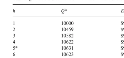
Table 3
Optimal order quantities and expected pro"t for di!erent dis-counting schemes and uniform demand distribution
h QHh E(n(h))
1 10000 $90,000.00
2 10460 $93,879.00
3 10587 $94,741.93
4H 10630 $94,804.75
5 10640 $94,544.00
6 10633 $94,123.15
7 10617 $93,613.39
Table 4
Optimal order quantities and expected pro"t for di!erent dis-counting schemes and normal demand distribution
h QH E(n(h))
1 10000 $91,999.97
2 10459 $95,466.63
3 10582 $96,550.64
4 10622 $96,939.17
5* 10631 $97,043.67
6 10623 $97,007.84
7 10607 $96,894.11
which can be solved using a simple search proced-ure. NowQH
h,h"1,2,nand their corresponding E(n(h)) are computed and the best QH
h is ordered.
EvaluatingE(n(h)) requires numerical integration.
Numerical Example 2.Reconsider Example 1 with
= uniformly distributed on [100, 140] which
im-plies thatx
0is uniformly distributed witha"8,000
andb"12,000 forP
0"$20. Using Eqs. (16) and
(17) gives the results in Table 3. Thus, the optimal number of prices is hH"4,QH"10,630 and
E(n(h))"$94,804.75. After the order is placed and demand becomes known, the application of Algo-rithm 1 may result in a new value of hH at the discounting problem. For smaller cost of discount-ing of F"$200, the solution changes to
hH"7,QH"10,797 andE(n(h))"$96,692.67. Suppose=is normally distributed with a mean
of E(=)"120 and standard deviation p(=)"10 which implies that x
0is normally distributed with
mean k
0"10,000 and standard deviation p"1,000 for P
0"$20. Using Eqs. (18) and (19)
gives the results in Table 4. Thus, the optimal number of prices is hH"5,QH"10,631, and
E(n(h))"$97,043.67.
5. Optimal initial price
In this case, initial unit o!ering price (P
0) is
a decision variable and the NV must determine the optimal values of bothQ andP
0. We analyze the
case of uniformly distributed demand (i.e.
x
0&U[a,b]) and provide closed-form solution for
it. Using P
0"C with the expressions for a and b gives the minimum and maximum possible de-mands, (=
Substituting from (20)}(23) into (16) gives
E(n(h))" b
Substituting di!erent values of h into (20) shows thata
1'0. Ifa2'0 then (26) gives one negative
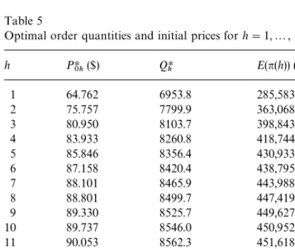
Table 5
Optimal order quantities and initial prices forh"1,2, 15
h PH0h($) QHh E(n(h)) ($)
1 64.762 6953.8 285,583
2 75.757 7799.9 363,068
3 80.950 8103.7 398,843
4 83.933 8260.8 418,744
5 85.846 8356.4 430,933
6 87.158 8420.4 438,795
7 88.101 8465.9 443,988
8 88.801 8499.7 447,419
9 89.330 8525.7 449,627
10 89.737 8546.0 450,952
11 90.053 8562.3 451,618
12 90.298 8575.4 451,780
13 90.489 8586.2 451,548
14 90.635 8595.0 451,004
15 90.746 8602.4 450,206
of a
3. If a2(0 and a3(0, (26) also gives one
negative root and one positive root. Ifa
2(0 and
a
3'0, (26) gives two positive roots. Eqs. (17) and
(26) can now be used in an iterative fashion until convergence to obtain the optimal quantity and price.
For normally distributed demand, we are unable to provide closed-form expressions forQH
h andPHh.
ForQ
hto be optimal, it must satisfy (19). ForPhto
be optimal it must satisfy dE(n(h))/dP"0, where
E(n(h)) is given by Eq. (18). Therefore, this case would require solving two nonlinear equa-tions until convergence for "nding QHh and
PHh,h"1,2,n. Numerical integration can then be
used to evaluate the correspondingE(n(h)) for each
hto identifyhH.
Numerical Example 3.Using the data of Example 1, Eqs. (17) and (26) converge to thePH0
h's andQHh's, h"1,2, 15 shown in Table 5 after 20 iterations
(actually convergence occurs in less than 20 iter-ations depending on the degree of precision re-quired).
From Table 5, the optimal order quantity is
QH"8575.4, the optimal initial o!ering price is
PH0"$90.23, the optimal number of prices is
hH"12 (which may change after demand becomes known), and the optimal expected pro"t is
E(n(h))"$451,780. Increasing the discounting cost
to F"$3,000 gives QH"8353,PH0"$85.82, and
hH"6, for whichE(n(h))"$411,530.
Reconsider Example 1 with uniformly distrib-uted=on [40, 80] which impliesx
0is uniformly
distributed with a"500 and b"1,500 at
P
0"$20. The demand function isP"=!0.04x,
which implies a 25 units increase in demand for each$1 drop in price. Eqs. (17) and (26) converge to
QH"1,014,PH0"$45.72, and hH"4, for which
E(n(h))"$18,296. Increasing the discounting cost to F"$1,500 gives QH"975,PH0"$43.58,
hH"3, for which E(n(h))"$16,368. Decreasing the discounting cost to F"$300 results in
QH"1,057,PH0"$48.40, and hH"6, for which
E(n(h))"$21,130.
6. Discussion and conclusion
In this paper, we extended the classical SPP to the case in which
1. demand is price dependent,
2. multiple discount prices are used to sell excess inventory,
3. the discount prices are under the control of the NV, and
4. there is a positive setup cost associated with discounting the product.
The resulting SPP is composed of two problems. In the "rst problem, after demand becomes known, the NV must determine the optimal discounting scheme. In the second problem, the NV must deter-mine the order quantity which maximizes the ex-pected pro"t prior to any demand being realized. Two algorithms were developed for solving the discounting problem under two di!erent assump-tions about the behavior of the NV. The order quantity problem was addressed for normal and uniform demand distributions. Furthermore, for cases where the initial price is also under the con-trol of the NV, the problem was solved for uniform demand distribution.
is more signi"cant for higher demand elasticity and smaller"xed discounting cost. The more elastic the demand, the larger the number of prices the NV should use and the smaller the di!erence between consecutive prices. The higher the"xed discounting cost, the smaller the number of prices the NV should use and the larger the di!erence between consecutive prices. Actually, the proposed model sheds some light on the behavior of retailers where multiple items are usually discounted together. By discount-ing multiple items together (such as all men's and/or women's apparel), the "xed discounting cost per item is reduced, the number of prices used to sell the items are increased, and revenue is increased.
The e!ect of the incorporation of multiple dis-counts on the optimal order quantity depends both on the elasticity of demand and the"xed discount-ing cost. From Eq. (17) one obtainsQH
h`1!QHh" P
0(h3!( 2h#1 )+hi/0~1i) /b h2(h#1 )2!F/P0.
Simple analysis shows that the "rst term to the right of the equality is positive and decreasing inh. Thus, the smaller the value ofband the smaller the
"xed discounting cost, the more likely that
QHh`1*QHh and that QHh`1 has higher expected pro"t thanQHh, especially at smaller values ofh. In this case, because demand elasticity is high and the
"xed discounting cost is low, the NV orders larger quantities knowing that any excess inventory can be sold by using small discounts without incurring a large"xed discounting cost.
Future research can address several extensions of the above model. An extension dealing with prices that are not equally spaced provides a useful gener-alization of the model. In this case, the NV only restricts the discounts to be at least a certain per-centage o!the original price so that customers see them as meaningful. The decision variables become the optimal prices (P0,P1,2,Pn) for the
discount-ing problem. Other extensions can deal with other types of demand}price relationships and other probability distributions of demand.
Acknowledgements
The author would like to thank the referees for their helpful suggestions. This work was supported, in part, by funds provided by the University of North Carolina at Charlotte.
Appendix A Subtracting (A.1) from (A.2) and simplifying gives
R
B(N)!RB(k)"
P
0
k(k!1)(x0!Q)(0, (A.3) which leads to a contradiction.
Proof of Lemma 2. From (8),
R Subtracting (A.5) from (A.4) and simplifying gives:
R For any discounting to be needed, Q'x
0 (or
equivalentlyP
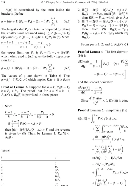
Table 6
brackets. De"ne
g"jv(v#1) (P The largest valueP
acan take is computed by taking
the smaller limit obtained usingP
a([(v!j#1)/ the upper limit on P
a is Pa"[(v!j#1)/v]P0
which when used in (A.7) gives the following expres-sion forg: The values of g are shown in Table 6. Thus
g"j(j!1)P and the second derivative
d2E(n(h)) Proof of Lemma 5. Simplifying (18) gives
The"rst and second derivatives of E(n(h)) are
Let y be normally distributed with mean k and standard deviationp. The probability distribution ofyis
f(y)" 1
J2npe~(y~k)
2@2p2
(A.13) with"rst derivative
f@(y)"!y!k
Substituting from (A.14) into (A.12) gives d2E(n(h))
provided in three parts:
1. From (A.15), a su$cient condition for d2E(n(h))/ dQ2)0 is
Fh(Q!iP
0/hb!k0)(P0p2, i"1,2,h!2.
(A.16)
which is satis"ed if
Fh(Q!k
0)(P0p2. (A.17)
By assumption 1, the largestFis atF"P20/bh2
which when substituted in (A.17) gives
Q(k
and the largest probability of obtaining this pro"t is [1!F
k(Q)]. Thus, an upper bound on G(Q) is
GU(Q)"k(P
0!C)[1!Fk(Q)]. (A.19)
For any value ofQ, the expected loss is
¸(Q)"(F#C!P which simpli"es to F
k(Q))0.5. Thus, QU) cient condition for optimality. Substituting for
QUandQC gives k
which simpli"es to the conditionkP20)b2h2p2
of the Lemma.
3. The smallest per unit pro"t in (A.18) is (P k!C)
and the smallest probability of obtaining this pro"t is [1!F
0(Q)]. Thus, a lower bound on
G(Q) is
GL(Q)"k(P
k!C)[1!F0(Q)]. (A.24)
Again an upper bound onQH, denotedQUis one which satis"esGL(Q)*¸(Q) which gives
k(P
k!C)[1!F0(Q)]*(F#C!Pk`1)Fk(Q).
(A.25) Simplifying (A.25) gives
k(P k!C) F#C!P
k`1
* Fk(Q)
1!F
0(Q)
. (A.26)
SinceF#C!P
k`1*k(P0!C),F#C!Pk`1 *k(P
k!C) and (A.26) becomes
1* Fk(Q)
1!F
0(Q)
. (A.27)
Since F0(Q)*F
k(Q),F0(Q) can be written as
F
0(Q)"Fk(Q)#DwhereD*0. Substituting in
(A.27) gives F
k(Q))(0.5!D/2). Thus, QU)
k
k"k0#kP0/hband the same argument
deal-ing with the largest expected gain can be applied
resulting in the condition kP20)b2h2p2 being su$cient.
References
[1] S. Nahmias, Production and Operations Management, Irwin, Boston, MA, 1996.
[2] G. Gallego, I. Moon, The distribution free newsboy prob-lem: Review and extensions, Journal of the Operational Research Society 44 (1993) 825}834.
[3] L.R. Weatherford, P.E. Pfeifer, The economic value of using advance booking of orders, OMEGA: International Journal of Management Sciences 22 (1994) 105}111. [4] T.M. Whitin, Inventory control and price theory,
Manage-ment Science 2 (1955) 61}68.
[5] E.S. Mills, Uncertainty and price theory, Quarterly Jour-nal of Economics 73 (1959) 116}130.
[6] A. Lau, H. Lau, The newsboy problem with price-dependent demand distribution, IIE Transactions 20 (1988) 168}175. [7] L.H. Polatoglu, Optimal order quantity and pricing
deci-sions in single-period inventory systems, International Journal of Production Economics 23 (1991) 175}185. [8] M. Khouja, The newsboy problem under progressive
mul-tiple discounts, The European Journal of Operational Re-search 84 (1995) 458}466.
[9] M. Khouja, A. Mehrez, A multi-product constrained news-boy problem with progressive multiple discounts, Com-puters and Industrial Engineering 30 (1996) 95}101. [10] M. Khouja, The newsboy problem with progressive
![table when there is a<last 3 will not be used since all inventory is soldis large. In addition, any discounting schemeshown in Table 2 for a given value ofxed cost of discountingapproximated using larger values ofall which may be proFor example, whences on the range [using six prices on the range [0,P P�, P�"�] may be approximated by"small quantity left and the " h may be h in Table 1."P�/2, using four pri- P�] (of which theprior to reaching those prices).](https://thumb-ap.123doks.com/thumbv2/123dok/3116668.1378604/5.544.28.240.48.146/inventory-discounting-schemeshown-discountingapproximated-approximated-quantity-theprior-reaching.webp)