A genetic algorithm to solve the general multi-level lot-sizing
problem with time-varying costs
N. Dellaert
!
, J. Jeunet
",
*
, N. Jonard
#,$
!Department of Operations Management, Eindhoven University of Technology, P.O. Box 513, 5600 MB Eindhoven, Netherlands "Laboratoire de Recherche en Gestion, Universite& Louis Pasteur, 61 Avenue de la ForeLt Noire, 67070 Strasbourg Cedex, France
#CNRS, Bureau d'Economie The&orique et Applique&e, 61 Avenue de la ForeLt Noire, 67070 Strasbourg Cedex, France $Maastricht Economic Research Institute on Innovation and Technology, P.O. Box 616, 6200 MD, Maastricht, Netherlands
Received 17 May 2000; accepted 14 June 2000
Abstract
The multi-level lot-sizing (MLLS) problem in material requirements planning (MRP) systems belongs to those problems that industry manufacturers daily face in organizing their overall production plans. However, this combina-torial optimization problem can be solved optimally in a reasonable CPU only when very small instances are considered. This legitimates the search for heuristic techniques that achieve a satisfactory balance between computational demands and cost e!ectiveness. In this paper, we propose a solution method that exploits the virtues and relative simplicity of genetic algorithms to address combinatorial problems. The MLLS problem that is examined here is the most general version in which the possibility of time-varying costs is allowed. We develop a binary encoding genetic algorithm and design "ve speci"c genetic operators to ensure that exploration takes place within the set of feasible solutions. An experimental framework is set up to test the e$ciency of the proposed method, which turns out to rate high both in terms of cost e!ectiveness and execution speed. ( 2000 Elsevier Science B.V. All rights reserved.
Keywords: Genetic algorithm; Lot-sizing; General product structure
1. Introduction
Material requirements planning (MRP) is an old
"eld of study within business, but it still plays an important part in coordinating replenishment deci-sions for complex"nished goods. There are actual-ly reasons to believe that the rise in consumers'
demands and expectations, and the subsequent in-crease in product complexity will make the need for
*Corresponding author.
E-mail address:[email protected] (J. Jeunet).
production coordinating devices even more accu-rate. However, we are not only in an era of rising product complexity but also in an era of "erce competition which de"nitely calls for adequate cost-saving tools. For this certainly MRP is not enough, as its basic philosophy is only to ensure that the right number of components is planned at the right time to meet the demand for end items. MRP therefore only provides a feasible solution to the multi-level production inventory problem, whereas ideally one would aim at a sequence of replenishment quantities through time at the vari-ous levels of manufacturing that keeps the total
relevant cost as low as possible while satisfying the demand for end items. Therefore, determining a proper lot-sizing policy de"nitely is a key dimen-sion of inventory control, as placing proper batches can allow for signi"cant reductions in inventory-related costs.
Optimal solution algorithms exist for this prob-lem [1], but only very small instances can be solved in reasonable computation time for the problem is NP-hard, not mentioning the mathematical com-plexity of the technique that might deter many potential users. Several approaches to solve vari-ants of the MLLS problem have been developed, with further assumptions made on the product and/or cost structure (see [2}5]), but execution times remain desperately high. Last, it should also be added that even when the time constraint is made as slack as possible, branch-and-bound algo-rithms available from standard software packages sometimes fail in"nding optimal solutions. Hence heuristic techniques that o!er a reasonable trade-o! between optimality and computational feasibility are highly advisable.
One alternative, which is often implemented in practice, consists in applying single-level decision rules }just like the economic order quantity }to each level of the product structure (see [6,7]). Though simplicity surely obtains, neglecting the fact that placing a lot for an item somewhere in the product structure often triggers lots for the sub-components of this item has dramatic conse-quences in terms of cost e!ectiveness. Of particular interest are the approaches in which the multi-level nature of the problem is explicitly taken into ac-count. Blackburn and Millen [8] suggested several cost modi"cations to account for interdependencies among levels of the product structure. Coleman and McKnew [9] developed a four-pass procedure based on the incremental part period algorithm (IPPA). The procedure embeds an original look-down routine used to compare at each level the net bene"t resulting from the lumping of each period's requirement, until the bottom of the product structure is reached. Contrary to both previous approaches, the method developed by Bookbinder and Koch [10] is not only designed to address pure assembly product structures but also general struc-tures, a feature being extremely common in real
settings. Dellaert and Jeunet [11] resort to ran-domization as a means of accounting for interde-pendencies among stages and achieve fairly good results compared to the previous techniques. How-ever, although these approaches usually outper-form sequential methods, they are unable to guarantee an optimal solution.
In this paper, we develop a hybrid genetic algo-rithm (GA) to solve the MLLS problem with no capacity constraints and no restrictive assumption on the product structure. Our primary incentive for this study is to "nd a solution method which is relatively moderate in CPU-time and intuitively appealing to potential users for a problem"eld of which Segerstedt [12] says &MRP and other methods without clear capacity constraints will no doubt continue to be used in practical installations for decades to come'. We consider the most general statement of the problem in which costs may vary from one time period to the next. Though the possibility of allowing time-varying costs could be considered a striking assumption, it should be re-called that the cost of carrying items in inventory includes the expenses incurred in running a ware-house, the costs associated with special storage requirements, deterioration, obsolescence and taxes, and primarily the opportunity cost of the money invested which is very likely to#uctuate as a result of changes in investment opportunities. Similarly, the set-up cost attached to replenishment decisions embeds learning e!ects (getting used to a new set-up, procedures and material has a cost in terms of scrap costs) and evolves in response to changes in the work force, especially when it is subject to frequent turnover.
Fig. 1. Three basic product structures. Larger instances con"rm the performance of the
GA, as it easily beats the sequential techniques we incorporated for the sake of comparison while keeping the computational demand extremely reasonable.
The paper is organized as follows. Section 2 is dedicated to the presentation and mathematical formulation of the MLLS problem. Section 3 gives the building blocks of the genetic algorithm: encod-ing, feasibility constraints, genetic operators and principles of evolution. Section 4 presents the ex-perimental framework and the parameter settings. Numerical results are discussed in Section 5 and in Section 6 conclusions and practical implications are derived.
2. The multi-level lot-sizing problem
In a manufacturing production system, end items are usually made up with a number of intermediate products which, in turn, consist in combinations of components (purchased parts and raw materials). Each end item is therefore described by a bill of materials, which is the product recipe. When con-sidering the issue of satisfying the demand for end items emanating from customers, the right quantity of each sub-component has to be made available at the right time, and if possible at the lowest cost. As products are associated with holding and set-up costs, di!erent inventory policies lead to di!erent costs and determining an optimal policy is a core concern.
The bill of materials is commonly depicted as a directed acyclic graph in which a node corres-ponds to an item and the edge (i, j) between nodes iandjexists if and only if itemiis directly required to assemble itemj. Itemiis fully de"ned byC~1(i) andC(i), the sets of its immediate predecessors and successors. The set of ancestors }immediate and non-immediate predecessors}of itemiis denoted
CK~1(i). Items are numbered in topological order by the integers 1,2,i,2,P so as to guarantee that any edge (i, j) satis"esj'i. Put another way, items are sorted in increasing level codes and each com-mon part is listed at the lowest level it appears in the product structure. Adopting the convention that"nished goods belong to level 0, items are then
numbered from 1 to P, starting the labeling from level 0 and moving sequentially to the lowest level. Hence, product 1 is always a"nished good whereas itemPis necessarily purchased.
Fig. 1 displays three types of product structures that are often encountered in the literature. Fig. 1(a) represents a pure assembly structure, in which every item has at most one direct successor (dC(i)3M0, 1N, for alli). By contrast, Fig. 1(b) shows a pure arborescent structure in which every item has at most one direct predecessor (dC~1(i) 3M0, 1N, for alli). Fig. 1(c) exhibits a general product structure for which C~1(1)"M2, 3N;CK~1(1)"
M2, 3, 4, 5N; C(4)"M2, 3Nand CK (4)"M1, 2, 3N. In this last structure, item 4 is commonly used by item 2 and 3, hence it is said to be a common part.
The MLLS problem consists in "nding a se-quence of lot sizes that minimizes the sum of set-up and inventory carrying costs, while meeting the demand for end items over a ¹-period planning horizon. To formulate the MLLS problem as a mixed integer program we use the symbols sum-marized in Table 1.
Our formulation follows that of Steinberg and Napier [1]. An optimal solution to the MLLS problem is obtained by minimizing
P + i/1
T + t/1
e
i,t)xi,t#si,t)yi,t#hi,t)Ii,t (1)
subject to the set of constraints
I
i,t"Ii,t~1#ri,t#xi,t!di,t, (2)
d i,t" +
j|C(i) c
i,jxj,t`lj, ∀iDC(i)O0, (3)
x
i,t!Myi,t)0, yi,t3M0, 1N, (4)
I
Table 1
Notations for the MLLS problem Cost parameters
s
i,t Set-up cost for itemiin periodt e
i,t Unit purchase or production cost for itemiin periodt h
i,t Unit inventory carrying cost per period for itemiin periodt Quantityvariables
d
i,t Gross requirements for itemiin periodt x
i,t Delivered quantity of itemiat the beginning of periodt I
i,t Level of inventory for itemiat the end of periodt r
i,t Scheduled receipts for itemiat the beginning of periodt y
i,t Boolean variable adressed to capturei's set-up cost in periodt Technical coezcients
l
i Lead time for itemi,
c
i,j Quantity of itemirequired to produce one unit of itemj(production ratio)
The objective function in Eq. (1) is the sum of purchase or production costs, set-up and inventory holding costs for all items over the planning hor-izon. Note that the possibility of time-varying unit purchase and production costs, inventory costs and set-up costs is allowed for. Eq. (2) expresses the#ow conservation constraint for item i. It de"nes the inventory level for itemiat the end of periodt. The variable I
i,0 is the initial level of inventory and
r
i,t designates the scheduled receipts, which result from previously made ordering decisions and rep-resent a source of the item to meet gross require-ments. Gross requirements consist in the external demand when end items are considered, and result from the lot sizes of immediate successors for com-ponent items, as stated in Eq. (3). We assume that no component is sold to an outside buyer, i.e. external demands only exist for "nished goods. Constraint (4), whereMis a large number, guaran-tees that a set-up cost will be incurred when a batch is purchased or produced. Finally, constraint (5) states that backlog is not allowed and that produc-tion is either positive or zero.
3. The genetic algorithm
In this section, we present the way a genetic algorithm can be customized to address the MLLS
problem. We "rst discuss the issue of encoding }
in our case a binary matrix representation}and the feasibility constraints. We then turn to the evolu-tionary stages of the algorithm and the speci"c genetic operators that have been designed to increase search e$ciency.
3.1. A binary matrix representation
The"rst issue that arises in designing a hybrid genetic algorithm is that of"nding a proper encod-ing. At this stage, we shall exploit a fundamental property of the MLLS problem that allows for a binary encoding. In the MLLS problem, costs are typically concave as a non-zero "xed cost is incurred whenever an order is launched (the set-up cost). Hence, though it might be optimal to place an order at a point in time where there are no net requirements, there is never more than one lot to cover a net requirement. Ordering more than once would imply extra costs (a formal proof is in Veinott [13]). Clearly if this was not the case, only real-coded or #oating-point genes could be employed, as quantities in each time period would have to be speci"ed. Hence, concavity implies that there is an optimal solution for which
x
Fig. 2. The decoding procedure. Knowing the list of delivery dates is therefore su$
-cient to derive ordered quantities. This leads to the most natural encoding which consists in represent-ing the list of delivery dates for all items as aP]¹ matrix
y"
A
y1,1 2 y1,T
F } F
y
P,1 2 yP,T
B
,
in whichy
i,t"1 if a set-up for itemiis delivered in period t, and y
i,t"0 otherwise. Searching for an optimal solution to the MLLS problem is therefore equivalent to "nding a binary matrixy such that the corresponding quantities minimize the objec-tive function (1). The vectory
i"(yi,1,2,yi,T) cod-ing order delivery dates for the scod-ingle itemiis called a string. Thus, in our setting, a chromosome yis a set of binary strings coding delivery dates for all items and periods.
For any chromosome, a decoding procedure is used to convert ordering dates into lot sizes, going sequentially from "nished goods to purchased items. This sequential procedure is based on the gross-to-net explosion process, a key element in MRP systems which translates product require-ments into component part requirerequire-ments, taking existing inventories and scheduled receipts into ac-count. Starting from the gross requirements (ex-ternal demand) for the end item, physical inventory is computed in each period. Physical inventory at the end of any period amounts to the inventory at the end of the previous period augmented with the scheduled receipts and reduced by the gross re-quirements. When this physical inventory falls below zero, we compute the net requirements, which are exactly what is needed to meet the gross
requirements. Lot sizes are such that they cover the net requirements. These lot sizes together with the technical coe$cients de"ne the gross requirements for any immediate component of the end item. These steps are summarized in Fig. 2.
As a brief illustration of how the decoding works, consider a stream of gross requirements d
i"(10, 15, 100, 20, 20), scheduled receipts r
i"(5, 0, 0, 0, 0) and an initial level of inventory I
i,0"12. We have zi"(7,!8,!108,!128, !148), hence net requirements equal b
i"(0, 8, 100, 20, 20), and the stringy
i"(1, 0, 1, 0, 0)"nally yieldsx
i"(8, 0, 140, 0, 0).
3.2. Feasibility
The check for feasibility follows a logic that is similar to that of the decoding procedure, starting from the end item and sequentially moving to lower levels. A chromosome is said to be feasible if and only if, for alli"1,2,P, the next two conditions are met:
(i) All net requirements for itemican be covered in time. This constraint refers to the possibility that any successor of item i can generate net requirements for itemi that simply cannot be covered, due to either itemi's lead time or item i's available quantities at the beginning of the horizon.
(ii) All net requirements for itemiare covered by proper set-ups. This constraint has to do with the consistency of the delivery dates y
i,t with the stream of net requirements for itemi.
To formally state condition (i), leta
Table 2
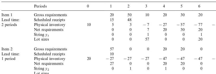
An example of indirect infeasibility
Periods 0 1 2 3 4 5 6 7
Item 1 Gross requirements 20 50 10 20 30 20 20
Lead time: Scheduled receipts 15 48
2 periods Physical inventory 10 5 3 !7 !27 !57 !77 !97
Lead time: Scheduled receipts 10
1 period Physical inventory 20 !27 !27 !27 !47 !47 !47 !47
Net requirements 27 0 0 20 20 0 0
Stringy
2 0 1 0 1 0 0 0
Lot sizes
scheduled receipts and lead times of itemi's compo-nents, a procedure whose presentation will be omit-ted for the sake of simplicity. Clearly, no order can take place beforea
i, and thus no net requirements should appear prior toa
i. This is written as To illustrate a case in which condition (i) fails, consider a "nished good (item 1) made from one single component (item 2) with a one-to-one pro-duction ratio. Consider the feasibility of chromo-somey"(y
1,y2) displayed in Table 2, in which we
also give the net requirements for item 1, the lot sizes resulting from stringy
1and the requirements
for item 2 computed from the lot sizes of item 1. As can be seen in Table 2, stringy
1implies a net
requirement of 27 units for item 2 in period 1 but this requirement cannot be covered due to the lead time of item 2. The "rst period in which it is pos-sible to receive ordered quantities of item 2 is
a2"2 if an order is launched in period 1. Thus, the possibility of lumping the "rst three net require-ments of item 1 into a lot in period 3 must be abandoned. Any chromosome embedding the stringy
1 will systematically be infeasible.
Let us now turn to the formal statement of condi-tion (ii). We shall "rst de"ne the sequence
Mt
i,w; w"1,2,=iNof strictly positive net require-ments dates for item i"1,2,P. Consider now stringy
i. As the"rst net requirement for itemihas
to be covered, there must be at least one set-up in the time interval betweena
iandti,1, whereti,1
de-notes the "rst period in which a positive net re-quirement appears for itemi. Due to the concavity assumption, we also know that it can never be opti-mal to cover a net requirement with more than one set-up. Hence between periodaiand periodt
i,1there
can be at most one set-up, which implies that there must be exactly one set-up betweenai andt
i,1, i.e. The concavity assumption actually implies that there cannot be more than one set up between any pair of dates t
i,w#1 and ti,w`1, that is to say
between any pair of consecutive requirements. But there might well be no set-ups at all between t
i,w#1 andti,w`1, as net requirements in period
t
i,w`1can be covered by a set-up anywhere between
that period and the"rst period in which a positive net requirement appears, and we know for sure that a set-up is necessarily ordered betweena
i andti,1.
Summarizing, this constraint is written as
ti,w`1
+ t/ti,w`1
y
i,t)1 for allw"1,2,=i. (9) The end of the planning horizon has a slightly di!erent status, as betweent
i,Wi#1 and¹the item is not required anymore, which implies that
T + t/ti,Wi`1
y
1Actually, it is enough to consider the lot-for-lot solution, for any other lumping would generate a last positive net require-ment prior tob
i.
2The stream of datesMu
jNobtains starting from the bottom of the product structure and proceeding from one level to the next, until level 0 is reached.
To illustrate condition (ii) consider again Table 2. Satisfaction of constraints (8)}(10) can easily be checked for item 1, with a1"3 and Mt
1,w;
w"1,2,=1N"M3, 4, 5, 6, 7N. Hence, though string y
1 meets condition (ii) the chromosome
y"(y
1,y2) is not feasible.
In order to further reduce the solution set, note that the last period in which an item is required might di!er from the last period of the planning horizon, and symmetrically the"rst possible period of production for any item usually does not co-incide with the "rst period of the horizon. This is ignored by the general MILP formulation of the MLLS problem but allows for substantial reduc-tions of the set of solureduc-tions. The option of releasing an order for purchased items in the "rst period must be considered (even if initial inventory levels cover the "rst net requirements) where costs are time-varying. Thus delivery of materials can at best start in period 1#l
i. Optimal delivery dates for purchased item i belong toM1#l
i,2, biN, where
b
i is the last period in which itemiis required.1As for a manufactured item, production can be in-itiated when all predecessors are simultaneously available. If we letu
jdenote the smallesttsuch as I
production of item 1 cannot be launched in period 2 since at this date no inventory of predecessor 3 is available. Thus, production is released in period 4 (4"maxM2, 4N) and becomes available at date 4#l
1"5. Hence, optimal delivery dates for
manufactured itemibelong to the set
G
lIn our genetic algorithm, only feasible chromo-somes will be considered. Each chromosome will have to pass the feasibility test before entering the
population. By doing so, we avoid the complication of de"ning sophisticated penalty functions to guide search and storing useless infeasible chromosomes in the population.
3.3. Genetic search operators
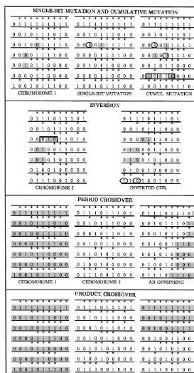
As there is no natural de"nition of genetic oper-ators for the MLLS problem with the binary rep-resentation we have adopted, we have designed"ve problem-speci"c search operators. When an oper-ator is applied to a feasible chromosome, it can happen that the altered chromosome is not feasible anymore. A simple repairing procedure is then ap-plied to make the chromosome anew feasible, by implementing adequate changes so that each string in the altered chromosome satis"es constraints (8)}(10). In case infeasibility arises from the viola-tion of constraint (7), the applicaviola-tion of the oper-ator is plainly cancelled. An example of how each operator works is given in the appendix.
3.3.1. Single-bit mutation
Mutation is usually de"ned as a change in a (ran-dom) number of bits in a chromosome. In our single-bit mutation, a unique bit undergoes muta-tion. This amounts to considering each chromo-some with given probability, selecting a random pair (iH,tH) such that iH3M1,2,PN and tH3Ma
iH,2,tiH,
WiHN, and changing its value from 0 to 1 or the opposite. This, in turn, can possibly trigger a series of changes in di!erent places in the chromosome in order to maintain its feasibility.
The mutated string should satisfy constraints (8)}(10). If mutation takes place in Ma
iH,2,t
iH,1N,
a symmetric mutation has to be performed in this same interval so as to ensure that there is exactly one set-up between aiH and tiH,1 as stated in
con-straint 8. Consider nowtH3Mt
iH,w#1,2,tiH,w`1N,
for w"1,2,=iH!1. When yiH,tH"0, there are
two possibilities. If there is already a bit equal to&1'
in this interval, it is swapped withy iH,
tH; otherwise,
y iH,
tHcan be set to 1 without violating the feasibility
constraint (9). Wheny iH,
tH"1, we know that there
Fig. 3. Parentsyandy@for crossover.
3It should be noted that in the numerical experiments we conducted, illegal o!springs never appeared.
Violation of constraint (7) for any ancestor entails the selection of a new random pair (iH,tH).
3.3.2. Cumulative mutation
Cumulative mutation performs the same muta-tion on the immediate predecessors of the item under consideration, with a lead time correction. The underlying intuition is that when mutation is performed on a given item, it might be worth changing the set-up periods for the predecessors, to account for product interdependencies. The repair-ing procedure is applied when necessary.
3.3.3. Inversion
We implement the following inversion. A ran-dom pair (iH,tH) is selected andy
exactly one of its neighbors di!er, we exchange their values. When both neighbors are di!erent from y
iH,
tH, one of them is randomly selected for
exchange. The same inversion is performed on item iH's predecessors. We "nally apply the repairing procedure to the altered chromosome.
3.3.4. Period crossover
The classical crossover is a one-point crossover that combines two chromosomes on the basis of one cross site randomly selected. Genetic material is swapped between two chromosomes to produce a pair of o!springs. Our crossover is a period cross-over that chooses a point in time tH randomly selected in the planning horizon. To produce o! -springs, we combine the"rst periods of one parent's strings with the last periods of the second parent's strings, the appropriate corrections being made when cumulative lead times have to be incorpor-ated (more details are given in the appendix). Again, we apply the repairing procedure when ne-cessary.
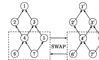
3.3.5. Product crossover
In the product crossover operator, the crossing point is an item chosen at random. To illustrate the functioning of this speci"c crossover, let us consider the product structure in Fig. 3 and assume the crossing point iH is item 5. We can replace stringy
5byy@5in parentyonly ify@5"ts feasibility
conditions (8)}(10) (see Section 3.2), given the
stream of positive net requirements datesMt
5,wNin
parenty.
Assume we keep y
4 unchanged whereas y5 is
replaced by y@5. Strings (y
4,y@5) will generate new
requirements for item 7 for which there is little chance thaty
7still"ts conditions (8)}(10). As items
4 and 5 have an ancestor in common (item 7), it might be wise not only to replacey
5byy@5but also
(y
4,y6,y7) by (y@4,y@6,y@7) wheny@4meets the
feasi-bility conditions when datesMt
4,wNare considered. To produce an o!spring, crossing itemiHas well as all items with which it shares at least one ances-tor must have strings y@ that meet the feasibility conditions when dates Mt
wN in parent y are con-sidered. The corresponding streams from parenty@
then replace the original strings in parenty. A sec-ond o!spring can be produced the same way, pro-vided the symmetric condition is satis"ed. The crossover procedure ends with a check of feasibility condition (7).3
3.4. Evolution: Selecting,searching and stopping
The initial populationPis generated by repeated
application of the single mutation operator to the chromosome coding delivery dates for the lot-for-lot policy, a replenishment rule which consists in placing an order each time a net requirement appears. The evaluation of chromosomes is achieved through the computation of the asso-ciated cost. Once the decoding procedure has been applied to each chromosome in the population, valuesI
from the delivery dates given by chromosomeyis derived (according to Eq. (1)). On the basis of this
&anti-"tness' evaluation function, we build the probability for an individual to become a member of the next generation. Once the cost C(yH) asso-ciated with chromosome yH has been calculated, the probability for individualyHto be a member of the new population is
exp[!j(C(yH)!C
.*/)/(CM!C.*/)] +y|Pexp[!j(C(y)!C
.*/)/(CM!C.*/)]
, (11)
wherejis a positive constant,C
.*/"miny|PC(y) is
the lowest cost in the current population and CM"+
y|PC(y)/dPis the population average cost.
The re-scaling that CM and C
.*/ operate on costs
permits to focus on relative cost di!erences rather than absolute ones, hence avoiding extra parameter tuning when moving from one problem to another. The logistic formulation in expression (11) is in-spired from a type of strategy used to assign lifetime values for chromosomes in varying population size (see for instance [14]). Chromosomes of minimum cost have the largest probability to belong to the next generation, and the largerjis the more likely it is that they actually do so}hence the stronger the selective pressure is. We add a small amount of elitism to our GA by always keeping the best indi-vidual from one generation to the next.
Evolution then works as follows. The search operators are sequentially activated with given probabilities on the current population to produce recombined individuals which found the next generation. Selection then operates on the current population and the chosen chromosomes join the genetically modi"ed ones to form the new genera-tion. The rest of the evolution is cyclic repetition of the previous steps.
Two categories of termination conditions gener-ally exist, respectively based on the structure of the chromosomes (search stops if chromosomes become identical) and on the progress made by the algorithm in a prede"ned number of generations (if the improvement is smaller than some epsilon, search is terminated). In the problem we consider, convergence towards a single chromosome cannot be guaranteed, for the optimal solution may not be unique. Consequently, we use this second stopping rule, denoted GAHn, in which search stops if no
signi"cant improvement is recorded during the last ngenerations. As this rule hardly o!ers any control on computation time, we also consider the rule GAN in which search is terminated after a "xed number of generationsN.
4. Experimental design
The purpose of the following experiments is"rst to test the algorithm against optimality in small-sized MLLS problems. In order to derive optimal solutions, we have used Steinberg and Napier's formulation and tried to solve the resultant mixed integer linear program with the general algebraic modeling system (GAMS), a standard optimization package. We then performed simulations for me-dium-sized instances to assess the cost performance of the GA.
4.1. The test problems
Two sets of experiments were considered, in which we"rst compared the performance of the GA to solutions provided by GAMS for small instances (10 products over 12 periods) and then examined the performance of the algorithm for medium-sized product structures (involving 50 products) over ex-tended planning horizons. In both phases, product structures were de"ned in terms of complexity. We used the complexity index proposed by Kimms [15] which is de"ned in the following way. Recall products are numbered in topological order by the integers 1,2,P and let P(k) be the number of products at levelk, withk"0,2,K (K#1 is the depth of the structure). The total number of items obviously equals+Kk/0P(k), which by de"nition is alsoP. The most complex}in the sense of having the largest number of product interdependencies
}structure is obtained when each item enters the composition of all the items located at higher levels in the product structure. By contrast, the simplest structure obtains when each item enters the composition of exactly one item belonging to a higher level. Kimms [15] de"nes the complexity of a product structure as
C" A!A.*/ A
.!9!A.*/
4We did not consider a C-value of 1 as we believed the corresponding product structures would be too intricate to be realistic.
whereA"+Pi/1dC(i) is the actual number of arcs in the structure. There is of course a minimal num-ber of arcs such as the product structure is connec-ted, which we denoteA
.*/and is equal toP!P(0).
Conversely there is a maximum number of arcs denoted A
.!9 that the graph can contain, and
which is written as
A
Structures for which the number of arcs equals the minimum number of arcs (A"A
.*/) are
necessar-ily assembly structures with a zeroC-value, where-as structures such where-as A"A
.!9 satisfyC"1. The
C-index is therefore bounded from below and above, whereas the traditional index of Collier [16] is not.
4.1.1. First phase:Test against optimality
Obtaining optimal solutions within reasonable CPU is a pretty di$cult task, even for small instan-ces. The"rst test phase therefore only involved 10-item product structures over a 12-period planning horizon. We controlled the complexity index (C) so that it took values within the set
M0.00, 0.25, 0.50, 0.75N.4For the sake of clarity, we have set the number of end-itemsP(0) to one, al-though the GA can easily handle product struc-tures in which there are multiple "nished goods. Without loss of generality we assumed a one-to-one production ratio in each case and set the depth of the structure (K#1 in our formalism) to four levels throughout, a very reasonable value for 10-item structures. Demand in each period for the end item was randomly drawn from a uniform distribution ranging from 0 to 200. Similarly, initial inventories for all items were randomly chosen in the range [0, 200] and scheduled receipts were set to zero for all items in all periods, again without loss of gener-ality. Cost parameters were chosen so as to guaran-tee increasing set-up costs and decreasing holding costs along any branch of the product structure tree. This is in accordance with the standard as-sumptions of value-added holding costs and high-est set-up costs for raw materials needing major
transformations versus lowest-order costs for end items only requiring assembly. An order cost in the range [45, 55] and a holding cost varying from 0.04 and 0.07 were assumed for all purchased items, in each period. For all other items, costs satisfy
s
Finally, lead times were randomly chosen and set to either 0 or 1. For each value of the commonality index, we performed"ve replications of costs and demands, hence a total number of 4]5"20 problems was examined in the"rst phase.
4.1.2. Second phase:Performance evaluation for medium-sized problems
The second phase of the experiment involved larger product structures embedding 50 items and longer planning horizons (24 and 36 periods were considered). Again we set C3M0.00, 0.25, 0.50, 0.75N. We considered a unique end-item together with a one-to-one production ratio and a structure depth of 10 levels, a reasonable value given the number of components. Carrying costs were com-puted in terms of random echelon cost uniformly drawn over [0.2, 4], as in Afentakis and Gavish [17]). Set-up costs for each item in each period were randomly selected from a uniform distribution over [100, 120]. For each value of the commonality index set-up costs were then multiplied by a scaling factor so as to avoid the lot-for-lot and the unique-lot solutions. Demand in each period uniformly selected over [0, 180]. The planning horizon was set to 24 and 36 periods. All lead times were ran-domly set to either 0 or 1 period. We generated 5 tests (replications of costs and demands) for each value of the complexity indexCand planning hor-izon, hence a total of 4]2]5"40 cases was con-sidered in the second phase.
4.2. Parameters setting of the genetic algorithm and other lot-sizing rules
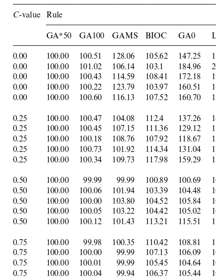
Table 3
Cost index values for GAMS and the various GAs for the small instances
C-value Rule
GAH50 GA100 GAMS BIOC GA0 L4L 0.00 100.00 100.51 128.06 105.62 147.25 162.51 0.00 100.00 101.02 106.14 103.1 184.96 205.94 0.00 100.00 100.43 114.59 108.41 172.18 199.81 0.00 100.00 100.22 123.79 103.97 160.51 191.05 0.00 100.00 100.60 116.13 107.52 160.70 182.92 0.25 100.00 100.47 104.08 112.4 137.26 143.74 0.25 100.00 100.45 107.15 111.36 129.12 131.25 0.25 100.00 100.18 108.76 107.92 118.67 120.51 0.25 100.00 100.73 101.92 114.34 131.04 134.11 0.25 100.00 100.34 109.73 117.98 159.29 170.49 0.50 100.00 99.99 99.99 100.89 100.69 100.89 0.50 100.00 100.06 101.94 103.39 104.48 105.15 0.50 100.00 100.00 103.80 104.52 105.84 106.87 0.50 100.00 100.05 103.22 104.42 105.02 106.04 0.50 100.00 100.12 101.43 113.21 115.51 117.58 0.75 100.00 99.98 100.35 110.42 108.81 110.42 0.75 100.00 100.00 99.99 107.13 106.09 107.13 0.75 100.00 100.01 99.99 105.45 104.64 105.45 0.75 100.00 100.04 99.94 106.37 105.44 106.37 0.75 100.00 100.00 100.00 105.67 103.48 105.67 generally acknowledged (see [18]) that further
in-creases in the population size do not necessarily lead to signi"cant improvements. The values of the number of generations for each stopping rule were based on intuitive and practical considerations (in-cluding numerous test runs).
In all experiments, we reported the results of rule GA0 (the initial population) in order to highlight the improvements reached within a positive num-ber of generations. The GA generally showed strong signs of cost convergence after 100 genera-tions in the smallest instances we considered. For larger problems we kept track of the performance of GA200 and GA300, and of course that of GAH50 which turned out to achieve the best overall results. Each of the"ve operators was applied with a con-stant probability equal to 0.1, and we arbitrarily set the selection parameterjin Eq. (11) to 25, which corresponds to a fairly strong selective pressure.
Though few heuristic methods have been de-signed for time-varying cost parameters, we had to incorporate some for the sake of comparison. We thus reported the lot-for-lot solution (L4L) that does not require any speci"c cost assumption to be implemented. We also considered the &best item ordering cycle' (BIOC) that consists in ordering each item every hperiod, wherehis the ordering cycle that leads to the minimum cost amongst costs associated with the various possible values of the ordering cycle (from one period to¹periods). Note that h obviously varies from one component to another.
5. Results
This section is devoted to the presentation and discussion of experimental data produced in the two test phases.
5.1. Small instances
Table 3 displays the results of the"rst test phase for eachC-value. Techniques are sorted in increas-ing cost order, the cost index beincreas-ing the ratio of the solution provided by each technique over the solu-tion provided by GAH50, which was used as a benchmark. Whenever a GA was used, we ran the
experiment 20 times in order to obtain statistically robust conclusions and reported the average value of the lowest cost individual over the 20 runs.
5That sometimes the cost ratio of GAMS to GAH50 is lower than 100 should be no surprise. The random generation of the initial population together with the particular sequence of ran-dom events shaping the search process create variability in the performance of the GA which sometimes keep it away from the optimal solution. There is however clear evidence that the GA is never far away.
quality, with cost di!erences that range from less than 1% up to 28%, and a 6.55% average excess cost rate.5The sequential BIOC algorithm stands out as a good compromise achieving a decent per-formance (7.7% excess cost on average) at the ex-pense of a negligible demand in computer time. Needless to say the lot-for-lot policy is outper-formed by all methods, with an excess cost rate approaching 36%. This is worse than the outcome of pure random search in the initial population GA0, which produces excess cost rates of about 28% (hence the magnitude of improvement).
Note how e$ciently GAH50 and GA100 have improved initial solution quality through selection and application of the"ve genetic operators. The fact that GAH50 outperforms GA100 is simply due to a longer search, for exploration goes on as long as it keeps paying o!.
Execution times are not given in detail in Table 3, for they were extremely low. The lot-for-lot policy and GA0 have negligeable requirements which never exceeded 0.005 seconds. The average CPU per replication amounts to 1.11 seconds for GAH50 (with standard deviation 0.22 seconds) and 0.72 seconds for GA100 (with standard deviation 0.03 seconds). (The longer execution times associated with GAH50 originate in the larger number of gen-erations that GAH50 performs, compared to GA100.) By contrast, GAMS reached solutions within the 5 minutes delay whose optimality was never guaranteed. We therefore end up with com-pletion times that, from a practical standpoint, are extremely reasonable and remain far away from the time spans required by GAMS for achieving low-quality solutions.
In order to get some insights into the workings of the GA, we also kept track of the performance of the "ve genetic operators involved in this study. For each operator we recorded the number of " t-ness improvements. We then computed the relative contribution of each operator to the total number
of improvements. Table 4 gives the success rates (in percent) obtained with GA100 and GAH50 in all test cases.
From Table 4 it is clear that search is not per-formed with equal e$ciency by all operators. The three mutation-based operators stand out in terms of successful search intensity whereas both cross-over exhibit lower rates. The reason for this is twofold. First, our crossovers participate in the process of variety creation, which is a key dimen-sion of evolutionary search. In the early stages of the process, they perform global search and gener-ate chromosomes that local search operators are likely to improve upon. Second, as the population converges, crossover tends to recombine identical chromosomes, which surely produces no improve-ment. By contrast, local search operators necessar-ily provoke changes, and thus have a chance to improve.
Before turning to larger cases, note that although standard optimization techniques can theoretically be employed to "nd an optimal solution to the MLLS problem, even in small-sized cases does the GA show its virtue, providing a quicker and better solution than GAMS. Supposedly, the tendency of the GA to outperform other techniques should be con"rmed when larger instances are considered.
5.2. Medium-sized problems
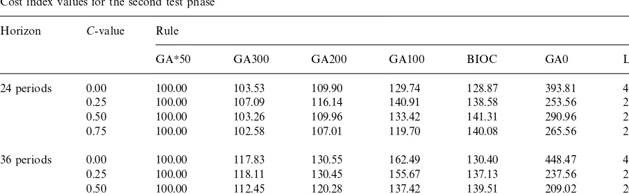
Table 5 summarizes the results of the second test phase. Techniques are arrayed by increasing cost order, the cost index being the ratio of the cost over the solution provided by GAH50, which was used as a benchmark. Each GA was replicated 10 times and the average minimum values are reported in Table 5.
The results of the second test phase con"rm the quality of GA-based techniques. Compared to the
Table 4
Relative rate of success for the"ve genetic operators in the GA
Rule C-value Genetic operators
Cumulative Period Product
mutation mutation Inversion crossover crossover
GA100 0.00 30.81 26.89 32.32 5.47 4.50
0.25 33.80 32.21 25.93 4.61 3.45
0.50 34.43 29.45 30.26 3.35 2.52
0.75 33.83 28.85 30.97 3.47 2.88
GAH50 0.00 31.61 28.59 32.09 4.22 3.49
0.25 34.83 34.70 24.63 3.14 2.70
0.50 34.75 34.65 25.03 2.70 2.87
0.75 33.39 33.23 28.89 2.63 1.86
Table 5
Cost index values for the second test phase Horizon C-value Rule
GAH50 GA300 GA200 GA100 BIOC GA0 L4L
24 periods 0.00 100.00 103.53 109.90 129.74 128.87 393.81 465.38
0.25 100.00 107.09 116.14 140.91 138.58 253.56 254.89
0.50 100.00 103.26 109.96 133.42 141.31 290.96 293.34
0.75 100.00 102.58 107.01 119.70 140.08 265.56 267.54
36 periods 0.00 100.00 117.83 130.55 162.49 130.40 448.47 496.18
0.25 100.00 118.11 130.45 155.67 137.13 237.56 238.40
0.50 100.00 112.45 120.28 137.42 139.51 209.02 209.74
0.75 100.00 116.38 125.86 147.29 149.54 293.95 295.64
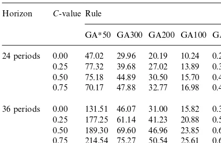
number of generations needed to reach a satisfac-tory outcome also rises. As expected, controlling the number of consecutive improvements leads to the best overall performances in spite of an addi-tional computaaddi-tional burden. Table 6 displays the time requirements of the GA at its various stages. We choose not to show the execution times of BIOC and of the L4L policy, as they remained steadily below 0.01 second in all the 40 test cases. By contrast, GAs are more greedy and CPUs in-crease with the number of generations, the max-imum value being attached to GAH50, the solution which also maximizes cost-e$ciency. Execution times are all increasing functions of the complexity index and the length of the planning horizon. Still,
with CPUs that are between half a minute and three minutes, GAs produce remarkably cost-e$ -cient solutions while formulating very reasonable computational demands. Although we chose not to report them here, it is worth mentioning that the success rates of the operators were approximately the same as in small instances.
Table 6
Execution time for the GAs in CPU seconds Horizon C-value Rule
GAH50 GA300 GA200 GA100 GA0 24 periods 0.00 47.02 29.96 20.19 10.24 0.25
0.25 77.32 39.68 27.02 13.89 0.35 0.50 75.18 44.89 30.50 15.70 0.40 0.75 70.17 47.88 32.77 16.98 0.45 36 periods 0.00 131.51 46.07 31.00 15.82 0.38 0.25 177.25 61.14 41.23 20.88 0.52 0.50 189.30 69.60 46.96 23.85 0.61 0.75 214.54 75.27 50.54 25.61 0.65
horizon length. Though we rejected the null hy-pothesis that GA100, GA200 and GA300 are equally e$cient under a 24 and a 36 periods hor-izon, both GA0 and GAH25 produce results which are not signi"cantly a!ected by the planning hor-izon. The relative performance of each rule is signif-icantly a!ected by complexity. The results are robust across the runs of the GA. They change substantially from a replication of costs and de-mands to another. This should be no surprise for there might be very di!erent product structures, as well as costs and demand patterns, for a given C-value.
6. Conclusion
Though the world of manufacturing is experienc-ing ongoexperienc-ing change both in terms of consumer needs and the organization of planning and control systems, a number of issues did not fade out. The necessity of carefully selecting adequate inventory control policies certainly is one of these issues. Solving the uncapacitated MLLS problem is left a daily concern for the vast majority of companies engaged in manufacturing production. But the computational requirements imposed by optimiz-ing routines tend to preclude their implementation in realistic size settings. Actually, despite the fact that the MLLS problem is encountered very often in practical installations, most solution methods are faced with severe di$culties in case the problem
size grows. One problem in selecting a lot-sizing procedure is that substantial reductions in inven-tory-related costs can generally be achieved only by using increasingly complex procedures. Optimal models not only demand mathematical prerequisite but also prove unable to solve problems pertaining to complex product structures. For time-varying cost parameters, there is even a lack of simple heuristic rules.
By contrast, the relative simplicity of the heuris-tic o!ered in this work, together with its cost-e$ciency, makes it an appealing tool to industrials, as documented by our simulation results. We designed speci"c genetic operators and purpose-fully constrained search to the set of feasible solutions. The "rst experimental test phase appraised the e!ectiveness of the GA in reference to the solutions provided by GAMS. In most cases the best performance was achieved by GAH50. Not only did the GA prove to be a very good cost-saving device, but it also maintained a computa-tional requirement much less stringent than that needed by GAMS. For larger problems, the GA again showed its ability to improve on initial solutions within reasonable time frames.
From a practical perspective, the heuristic of-fered in this work is signi"cantly easier to under-stand and implement than optimal mathematical methods. It o!ers a very satisfactory trade-o! be-tween algorithmic complexity and optimality, and as such we believe it can be a powerful near-optimal method for actual settings as well as a useful bench-mark to evaluate future heuristic methods.
Appendix. Example of operators
Let us consider the product structure in Fig. 3. Lead times Ml
iNi/1,2,7 equal M1, 1, 2, 0, 1, 1, 0N
and the gross requirements for item 1 (end item) over a 10-period horizon are given by
M200, 100, 20, 50, 10, 40, 65, 100, 40, 30N. Initial inventoriesMI
1,0,2,I7,0NequalM270, 100, 130, 200,
0, 0, 0N. All scheduled receipts are set to zero except for item 5 for which we haver
5,1"25. We assume
a one-to-one production ratio.
which correspond to feasible solutions to the problem with the general product structure in Fig. 3 over ten periods. Positive net requirements are symbolically represented by stars.
Assume the pair (iH,tH)"(3, 5) in chromosome 1 is selected for mutation. In thesingle-bit mutation, this triggers a mutation from 1 to 0 in period 3 to satisfy condition (7) as a single order is necessary to cover the"rst positive requirement (which occurs in period 5). In the cumulative mutation, the same mutations take place for item 3. We now perform a mutation from zero to one to items 4 and 5 (the predecessors of item 3) in period tH! l
iH"5!2"3. This entails a mutation from 1 to
0 for item 4 in period 5 to satisfy condition (7). Stringy
5is left unchanged sincey5,3already equals
one. String y
6 is no longer feasible since new net
requirements have been generated for this item. The "rst net requirement appears earlier than before and needs to be covered in time. Periods 2 and 3 are candidates for an order and period 2 is
"nally selected at random. There is now only one net requirement in time intervalM4, 5, 6Nbut two orders. One of them is selected at random for can-cellation. Bity
6,6 is therefore set to 0.
Assume the pair (iH,tH)"(3, 4) is selected for inversion. Bity
3,4 can either be swapped with bit
y
3,5 or bit y3,3. Suppose bit y3,5 is randomly
chosen for swapping. Bity
3,4 then takes the value
of y
3,5 which is zero and bit y3,4 is set to one.
Predecessors of item 3, say items 4 and 5, undergo the same inversion in periodstH!l
3"4!2"2
and its neighbouring period 3. Bitsy
4,2andy5,2are
respectively, swapped withy
4,3andy5,3. The
inver-sion leads to new requirements for item 7 and some mutations have to be performed to satisfy the feasi-bility conditions.
Fig. 4 exhibits an example of period cross-over when the crossing site is period 9. The"rst string of the o!spring combines the"rst 9 ordering periods for item 1 in chromosome 2 and the last ordering period of item 1 in chromosome 1. Let tHi be the crossing period for item i. We have tH1"9. The crossing period for any other itemi(i'1) is given bytH
that each string in the o!spring is feasible regarding the new positive requirements.
Assume item 5 is selected as a crossing point to implement the product cross-over. To produce an o!spring, we simply combine (y
1,y2,y3) from
chro-mosome 1 with strings (y
4,y5,y6,y7) from
chromo-some 2. One can easily check the feasibility of the resultant o!spring. Let us note that the symmetric o!spring is not feasible.
References
[1] E. Steinberg, H.A. Napier, Optimal multi-level lot sizing for requirements planning systems, Management Science 26 (1980) 1258}1271.
[2] W.I. Zangwill, Minimum concave cost#ows in certain networks, Management Science 14 (1968) 429}450. [3] W.I. Zangwill, A backlogging model and a multi-echelon
model of a dynamic economic lot size production system
} a network approach, Management Science 15 (1969) 506}527.
[4] W.B. Crowston, H.M. Wagner, Dynamic lot size models for multi-stage assembly systems, Management Science 20 (1973) 14}21.
[5] P. Afentakis, B. Gavish, U. Karmarkar, Computationally e$cient optimal solutions to the lot-sizing problem in multistage assembly systems, Management Science 30 (1984) 237}249.
[6] L.E. Yelle, Materials requirements lot sizing: A multi-level approach, International Journal of Production Research 17 (1979) 223}232.
[7] E.A. Veral, R.L. LaForge, The performance of a simple incremental lot-sizing rule in a multilevel inventory envi-ronment, Decision Sciences 16 (1985) 57}72.
[8] J.D. Blackburn, R.A. Millen, Improved heuristics for multi-stage requirements planning systems, Management Science 28 (1982) 44}56.
[9] B.J. Coleman, M.A. McKnew, An improved heuristic for multilevel lot sizing in material requirements planning, Decision Sciences 22 (1991) 136}156.
[10] J.H. Bookbinder, L.A. Koch, Production planning for mixed assembly/arborescent systems, Journal of Opera-tions Management 9 (1990) 7}23.
[11] N.P. Dellaert, J. Jeunet, Randomized cost-modi"cation procedures for multi-level lot-sizing heuristics, Research Report TUE/BDK/LBS/99-02, Eindhoven University of Technology, 1999.
[12] A. Segerstedt, A capacity-constrained multi-level inven-tory and production control problem, International Jour-nal of Production Economics 45 (1996) 449}461. [13] A.F. Veinott Jr., Minimum concave-cost solution of
Leontief substitution models of multifacility inventory systems, Operations Research 17 (1969) 262}291. [14] Z. Michalewicz, Genetic Algorithms#Data Structures
[15] A. Kimms, in: Multi-Level Lot-Sizing and Scheduling Methods for Capacitated, Dynamic, and Deterministic Models, Physica Verlag Series on Production and Logis-tics, Springer, Berlin, 1997.
[16] D.A. Collier, The measurement and operating bene"ts of component part commonality, Decision Sciences 12 (1981) 85}96.
[17] P. Afentakis, B. Gavish, Optimal lot-sizing algorithms for complex product structures, Operations Research 34 (1986) 237}249.