SEMANTIC SEGMENTATION OF FOREST STANDS OF PURE SPECIES AS A GLOBAL
OPTIMIZATION PROBLEM
Cl´ement Dechesne, Cl´ement Mallet, Arnaud Le Bris, Val´erie Gouet-Brunet
Univ. Paris-Est, LASTIG MATIS, IGN, ENSG, F-94160 Saint-Mande, France [email protected]
Commission II, WG II/6
KEY WORDS:Forest stands, classification, regularization, semantic segmentation, graph-cut, graphical models, MRF, CRF.
ABSTRACT:
Forest stand delineation is a fundamental task for forest management purposes, that is still mainly manually performed through visual inspection of geospatial (very) high spatial resolution images. Stand detection has been barely addressed in the literature which has mainly focused, in forested environments, on individual tree extraction and tree species classification. From a methodological point of view, stand detection can be considered as a semantic segmentation problem. It offers two advantages. First, one can retrieve the dominant tree species per segment. Secondly, one can benefit from existing low-level tree species label maps from the literature as a basis for high-level object extraction. Thus, the semantic segmentation issue becomes a regularization issue in a weakly structured environment and can be formulated in an energetical framework. This papers aims at investigating which regularization strategies of the literature are the most adapted to delineate and classify forest stands of pure species. Both airborne lidar point clouds and multispectral very high spatial resolution images are integrated for that purpose. The local methods (such as filtering and probabilistic relaxation) are not adapted for such problem since the increase of the classification accuracy is below 5%. The global methods, based on an energy model, tend to be more efficient with an accuracy gain up to 15%. The segmentation results using such models have an accuracy ranging from 96% to 99%.
1. INTRODUCTION
The analysis of forested areas from a remote sensing point of view can be performed at three different levels: pixel, object (mainly trees) or stand. When a joint mapping and statistical reasoning is required (e.g., land-cover (LC) mapping and forest inventory), forest stands remain the prevailing scale of analysis (Means et al., 2000, White et al., 2016). A stand can be defined in many different ways in terms of homogeneity: tree specie, age, height, maturity, and its definition varies according to the coun-tries. Most of the time in national forest inventories, for reliability purposes, each area is manually interpreted by human operators using very high resolution (VHR) geospatial images with a near infra-red channel (Kangas and Maltamo, 2006).
Among the large body of available remote sensing data today, airborne laser scanning (ALS) and Very High spatial Resolution (VHR) hyper/multispectral images are both well adapted and com-plementary inputs for stand segmentation (Dalponte et al., 2012, Dalponte et al., 2015, Lee et al., 2016). ALS provides a direct access to the vertical distribution of the trees and to the ground underneath. Hyperspectral and multispectral images are particu-larly relevant for tree species classification: spectral and textural information from VHR images can allow a fine discrimination of many species, respectively. Multispectral images are often pre-ferred due to their higher availability, and higher spatial resolu-tion. One should note that the literature remains focused on indi-vidual tree extraction and tree species classification, developing site-specific workflows with similar advantages, drawbacks and classification performance. Consequently, no operational frame-work embedding the automatic analysis of remote sensing data has been yet proposed in the literature for forest stand segmenta-tion (Dechesne et al., 2017). More surprisingly, only few methods have addressed such an issue from a research perspective. More
authors have focused on forest delineation (Eysn et al., 2012), that do not convey information about the tree species and their spatial distribution.
The analysis of the lidar and multispectral data is performed at three levels in (Tiede et al., 2004), following the hierarchy of the nomenclature of forest LC species database. The multi-scale analysis offers the advantage of alleviating the standard limita-tions of individual tree crown detection, and of retrieving labels related here to forest development stage. Nevertheless, the pipeline is highly heuristic and under-exploits lidar data. Besides, signifi-cant confusions between classes are reported.
The automatic segmentation of forests in (Diedershagen et al., 2004) is also performed with lidar and VHR multispectral im-ages. The idea is to divide the forests into higher and lower sections according to the height provided by the lidar sensor. An unsupervised classification process is applied and pre-defined thresholds enable to obtain the desired delineation of stands. This method is efficient if the canopy structure is homogeneous and requires a strong knowledge on the area of interest. Based on height information only, it cannot differentiate two stands of sim-ilar height but different species.
Eventually, in (Dechesne et al., 2017), forest stand segmentation is considered from semantic segmentation point of view. For-est areas are first classified according to the tree species at the pixel and tree levels using lidar and multispectral airborne im-ages. Then, the label map is smoothed using an energetic frame-work that integrates both lidar and optical features.
In this paper, we specifically focus on semantic segmentation of forest stands through the regularization/smoothing process of an existing label map of pure species, following the strategy pro-posed in (Dechesne et al., 2017). Therefore, we build upon the vast amount of literature dealing with tree species classification at the tree level and investigate how the combined use of airborne lidar and VHR multispectral images can provide more accurate label maps. Simple smoothing methods are first investigated as well as more complex energy formulations. We aim to determine whether a complex formulation of the problem helps to obtain better results in such non-structured environments.
2. RELATED WORKS
2.1 How to smooth a label map?
Pixel-wise classification is not sufficient for both accurate and smooth land-cover mapping with VHR remote sensing data. This is particularly true in forested areas: the large intra-class and low inter-class variabilities of classes result in noisy label maps at pixel or tree levels. This is why various regularization solu-tions can be adopted from the literature (from simple smoothing to probabilistic graphical models, see Section 2.1).
According to (Schindler, 2012), both local and global methods can provide a regularization framework, with their own advan-tages and drawbacks. In local methods, the neighborhood of each element is analyzed by a filtering technique. The labels of the neighboring pixels (or the posterior class probabilities) are com-bined so as to derive a new label for the central pixel. Majority voting, Gaussian and bilateral filtering can be employed if it is not targeted to smooth class edges.
Global methods consider the full area of interest at the same time. They are based on Markov Random Fields (MRF), the labels at different locations are not considered to be independent. The op-timal configuration of labels is retrieved when finding the Maxi-mum A Posteriori over the entire field (Moser et al., 2013). The problem is therefore considered as the minimization procedure of an energyEover the full imageI. Despite a simple neighbor-hood encoding (pairwise relations are often preferred), the opti-mization procedure propagates over large distances. Depending on the formulation of the energy, the global minimum may be reachable. However, a large range of optimization techniques allow to reach local minima close to the real solution, in par-ticular for random fields with pairwise terms (Kolmogorov and Zabih, 2004). For genuine structured predictions, in the fam-ily of graphical probabilistic models, Conditional Random Fields (CRF) have been massively adopted during the last decade. Inter-actions between neighboring objects, and subsequently the local context can be modelled and learned. In particular, Discrimina-tive Random Fields (DRF, (Kumar and Hebert, 2006)) are CRF defined over 2D regular grids, and both unary/association and bi-nary/interaction potentials are based on labelling procedure out-puts. Many techniques extending this concept or focusing on the learning or inference steps have been proposed in the literature (Kohli et al., 2009, Ladick´y et al., 2012). A very recent trend
even consists in jointly considering CRF and deep-learning tech-niques for the labelling task (Kirillov et al., 2015).
In standard LC classification tasks, global methods are known to provide significantly more accurate results (Schindler, 2012) since contextual knowledge is integrated. This is all the more true for VHR remote sensing data, especially in case of a large number of classes (e.g., 10, (Albert et al., 2016)), but presents two disadvantages. For large datasets, their learning and infer-ence steps are expensive to compute. Furthermore, parameters should often be carefully chosen for optimal performance, and authors that managed to alleviate the latter problem still report a significant computation cost (Lucchi et al., 2011).
2.2 Semantic segmentation is a suitable solution
The classification process can be eased with segmentation tech-niques. Such algorithms provide strong local spatial supports (namely superpixels), sometimes at various scales (Lucchi et al., 2011). This is the so-called Object-Based Image Analysis (OBIA) framework. A pure bottom-up process is however not sufficient in our case. Alternatively, it can be achieved with more sophis-ticated top-down processes, e.g., based on pattern recognition methods but, emphasis is then put on localization of the objects of interest instead of sharp boundary retrieval (i.e., the reverse advantage of per-pixel classification). The best of both worlds is obtained with semantic segmentation, which aims to solve the in-terleaved issue of classification and segmentation by combining top-down and bottom-up cues. It defines the task of partition-ing an image into regions that delineate meanpartition-ingful objects and labelling those regions with an object label. While it is very pop-ular in computer vision (Ladick´y et al., 2010, Boix et al., 2011, Arbel´aez et al., 2012, Chen et al., 2015), it has been barely ad-dressed in the remote sensing community (Montoya-Zegarra et al., 2015, Zheng and Wang, 2015). Segmentation segmentation frameworks have demonstrated their usefulness in particular in structured environments such as urban areas. Emphasis is put on context learning in (Volpi and Ferrari, 2015) and on the design of robust yet locally discriminative modelling strategy for urban area classification of VHR multispectral images. It is based on a flexible energetical framework, namely a CRF. The adoption of fully-connected CRF can even allow to learn longer class inter-actions such as shown in (Li and Yang, 2016). Finally, seman-tic segmentation can be achieved using Deep Neural Networks, assuming the standard procedure is accompanied with proper de-convolution steps or with a Fully Connected Network such as in (Marmanis et al., 2016).
In forested areas, the combined use of airborne lidar (for height structure) and VHR multispectral images (for species composi-tion) into such a smoothing process would allow (i) to retrieve ho-mogeneous patches, (ii) to define the homogeneity criterion/criteria and (iii) to control the level of generalization of the final label map.
3. METHODS
3.1 General strategy
extracted both from 3D lidar point clouds and aerial multispec-tral images. The training pixels are selected according to an ex-isting forest LC geodatabase. The used classifier is the Random Forest (RF) classifier. This is an efficient classifier, that directly handles multiple classes, and provides posterior probabilities for each class.
Here, both local and global methods are tested. For local tech-niques, majority voting and probabilistic relaxation are selected (Sections 3.2 and 3.3). For global methods, various energy for-mulations based on a feature-sensitive Potts model are proposed (Section 3.4).
3.2 Filtering
An easy way to smooth a probability map is to filter it. All the pixels in ar×rpixels moving windowWare combined in order to generate an output label of the central pixel. The most popular filter is the majority filter. Firstly, the class probabilities are con-verted into labels, assuming that the label of pixelxis the label of the most probable class.
C(x) = [ci|P(x, ci)≥P(x, cj)∀j], (1) withi, j∈[1, nc], wherencis the number of classes. From this
label image, the final smoothed result is obtained by taking the majority vote in a local neighborhood.
Csmooth(x) =arg max
Many other filters have been developed but are not investigated in this paper.
3.3 Probabilistic relaxation
The probabilistic relaxation aims at homogenizing probabilities of a pixel according to its neighboring pixels. The relaxation is an iterative algorithm in which the probability at each pixel is up-dated at each iteration in order to have it closer to the probabilities of its neighbors (Gong and Howarth, 1989). It was adopted for simplicity reasons. First, good accuracies are reported with de-cent computing time, which is beneficial over large scales. Sec-ondly, it offers an alternative to edge aware/gradient-based tech-niques that may not be adapted in semantically unstructured envi-ronments like forests. The probabilityPt
k(u)of classkat a pixel uat the iterationtis defined byδPt
k(u)which depends on:
• The distancedu,vbetween the pixeluand its neighborsv (the pixels that are distant of less thanrpixels fromu).
• A co-occurrence matrixTk,ldefining a priori correlation
be-tween the probabilities of neighboring pixels. The local co-occurrence matrix has been tuned arbitrarily, but can also be estimated using training pixels (Volpi and Ferrari, 2015). The matrix is expressed as follow:
Tk,l=
The update factor is then defined as:
δPkt(u) =
In order to keep the probabilities normalized, the update is per-formed in two steps using the unnormalized probabilityQt+1
k (u)
The global smoothing method uses only a small number of pair-wise cliques between neighboring pixels (4-neighbors or 8-neighbors) to describe the smoothness. Over the entire resulting first order random fields, the maximization of the posterior probability leads to a smoothed results. This can be done by finding the minimum of the negative log-likelihood, arg min
C values of the features at pixelu(such as height, reflectance...) andNuis the 8-connected neighborhood of the pixelu(only the
8-connected neighborhood is investigated in this paper). When γ= 0, the pairwise term has no effect in the energy formulation; the most probable class is attributed to the pixel, leading to the same result as the classification output. Whenγ6= 0, the result-ing label map becomes more homogeneous, and the borders of the segments/stands are smoother. However, ifγis too high, the small areas are bound to be merged into larger areas, removing a part of the useful information provided by the classification step. The automatic tuning of the parameterγ has been addressed in (Moser et al., 2013) but is not used here.
In this paper, two formulations ofEdata(unary term) and four for-mulations ofEpariwise(prior) are investigated.
3.4.1 Unary term A widely used formulation for the unary term is the log-inverse formulation using the natural logarithm. It corresponds to the information content in information theory and is formulated as follow:
Edata=−log(P(u)). (7) It highly penalizes the low-probability classes but increase the complexity with potential infinite values.
An other simple formulation for the unary term is the linear for-mulation,
Edata= 1−P(u). (8) It penalizes less than the log-inverse formulation but has the ad-vantage of having values lying in[0,1].
thePotts modelis:
Epairwise(C(u) =C(v)) = 0, Epairwise(C(u)6=C(v)) = 1.
(9)
In thez-Potts model, the penalty for a change of label depends on the gradient of height between two neighboring pixels. The z-Potts modelis a standardcontrast-sensitive Potts modelapplied to the height obtained from the point clouds. Here, since we are dealing with forest stands that are likely to exhibit distinct heights, the gradient of the height map (given with the 3D lidar point cloud) is computed for each of the four directions sepa-rately. The maximumMg over the whole image in the four
di-rections is used to compute the final pairwise energy. A linear function has been used: the penalty is highest when the gradient is 0, and decreases until the gradient reaches its maximum value. The prior of thez-Potts modelis therefore:
Epairwise(C(u) =C(v)) = 0,
absolute value of the height difference of the two pixels. An other pairwise energy investigated is a global feature sensitive energy (called hereExponential-features model). The pairwise energy is computed with respect to a pool ofnfeatures. When the features have close values, the penalty is high and decreases when the features tends to be very different. The pairwise energy in this case is expressed as follows:
Epairwise(C(u) =C(v)) = 0, pute such energy, the features need to be first normalized (i.e., zero mean, unit standard deviation) in order ensure that they all have the same dynamic.
The last formulation investigated is also a global feature sensitive energy (called hereDistance-features model). The pairwise en-ergy is still computed with respect to a pool ofnfeatures. In this case, the energy is computed according to the distance between the two neighboring pixels in the feature space, the penalty is high when the pixels are close in the feature space and decrease when they get distant. The pairwise energy in this case is expressed as follow:
To compute such energy, the features need to be first normalized (i.e., zero mean, unit standard deviation) in order ensure that they all have the same dynamic. They are then rescaled between0and 1to ensure that||A(u);A(v)||n,2lies in[0; 1]∀(u,v).
In (Dechesne et al., 2017), a high number of features was ex-tracted from available lidar and optical images (∼100) but can be selected. They can also be weighted according to their
impor-tance, computed through the Random Forest classification pro-cess. Since the most important features (20) are almost all equally weighted, it does not bring additional discriminative information for the global feature sensitive energy.
3.4.3 Energy minimization The energy minimization is per-formed using graph-cut methods. The graph-cut algorithm em-ployed is the quadratic pseudo-boolean optimization (QPBO). The QPBO is a popular and efficient graph-cut method as it ef-ficiently solves energy minimization problems (such as the pro-posed ones) by constructing a graph and computing the min-cut (Kolmogorov and Rother, 2007). α-expansion moves are used, as they are an efficient way to deal with the multi-class problems (Kolmogorov and Zabih, 2004).
4. DATA AND RESULTS
4.1 Data
The different smoothing methods have been conducted on 4 moun-tainous test areas. Each area has a surface of 1 km2. The IRC ortho-images of the test areas are presented in Figure 1. The pro-posed areas exhibit a large range of species (>4). The airborne multispectral images were captured by the IGN digital cameras (Souchon et al., 2012). They have 4 bands: 430-550 nm (blue), 490-610 nm (green), 600-720 nm (red) and 750-950 nm (near infra-red) at 0.5 m ground sample distance (spatial resolution). The airborne lidar data were collected using an Optech 3100EA device. The footprint was 0.8 m in order to increase the probabil-ity to reach the ground. The point densprobabil-ity for all echoes ranges from 2 to 4 points/m2
. Our multispectral and lidar data fit with the standards used in many countries for large-scale operational forest mapping purposes (White et al., 2016). The multispectral images and the lidar data were acquired simultaneously.
(a) Area 1 (1 km2). (b) Area 2 (1 km2).
(c) Area 3 (1 km2). (d) Area 4 (1 km2).
4.2 Results
The results for all methods are presented for Area 2 in Table 1. The overall accuracy is computed by comparing the labelled pix-els in the forest LC, to the pixpix-els of the output images. The fil-tering method performs the worse with a gain of less than 1% compared to the classification, even with large filters. Further-more, the larger the filter is, the longer are the computation times. The probabilistic relaxation has also poor results (+5% than the classification) and has also important computation times, since the iterative process runs until the convergence has been reached. The global smoothing methods have great results, increasing the accuracy up to 15%. Thez-Potts modeltends to have slightly worse results than the other methods. ThePotts modeland the Distance-features modelhave very close results regardless of the unary term. The Exponential-features modelhave the greatest results with the linear unary, but have poor results with the log-inverse unary. It appears that it is the only energy that is sensitive to the unary term, indeed, for thePotts model, thez-Potts model and theDistance-features model, the difference between the lin-ear unary and the log-inverse unary is less than 0.2%.
Methods Smoothing Parameter
overall accuracy
Filtering 82.33% r= 5
Filtering 82.41% r= 25
Probabilistic relaxation 86.89% r= 5
Potts
Table 1. Results for the proposed methods for Area 2. The classification has an overall accuracy of 81.41%.
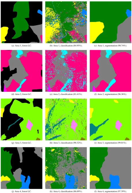
The best results for the four areas are presented in Figure 2. It shows that the proposed formulation is very efficient to retrieve forest patches of pure species with smooth borders. The accuracy ranges from 96% to 99%. Furthermore, the borders between ad-jacent classes fit well with the ones from the forest LC borders,
which validates the relevance of our model. However, in areas where no data is available, it is hard to ensure that our model has relevant results, but, from a visual point of view, the results seem good.
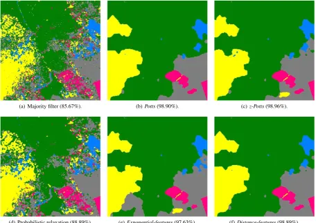
The results for all the proposed models using the log-inverse unary are presented for Area 1 in Figure 3. It appears clearly that ba-sic methods (such as filtering or probabilistic relaxation) are not adapted to our problem since the results remain very noisy. How-ever, having a too binding unary term in the model also leads to noisy results. Even if the accuracy is higher than the accuracy using the linear unary, the small patches produced with the log-inverse unary are not acceptable for a forest LC.
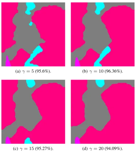
The effect of the parameterγis presented in Figure 4. Whenγis low, the borders are rough and small regions might appear (Fig-ure 4(a)). Increasingγsmooth the borders, however, a too high value have a negative impact on the results, reducing the size of meaningful segments (Figure 4(c)) or even removing them (Fig-ure 4(d)). The tuning of the parameterγis an important issue, since different values ofγmight be acceptable depending on the level of detail expected for the segmentation. In forest inven-tory, having small regions of pure species is interesting for the understanding of the behavior of the forest. For generalization purposes (such as forest LC), the segments must have a decent size and may exhibit variability.
(a)γ= 5(95.6%). (b)γ= 10(96.36%).
(c)γ= 15(95.27%). (d)γ= 20(94.09%).
Figure 4. Results of theExponential-features modelwith linear unary for different values ofγfor Area 2, the overall accuracy is
specified in brackets. Color codes: deciduous oaks, fir or spruce, chestnut, robinia.
5. CONCLUSION
(a) Area 1, forest LC. (b) Area 1, classification (84.95%). (c) Area 1, segmentation (98.74%).
(d) Area 2, forest LC. (e) Area 2, classification (81.41%). (f) Area 2, segmentation (96.36%).
(g) Area 3, forest LC. (h) Area 3, classification (90.32%). (i) Area 3, segmentation (99.01%).
(j) Area 4, forest LC. (k) Area 4, classification (86.69%). (l) Area 4, segmentation (97.39%).
Figure 2. Results for all the 4 areas, the overall accuracy is specified in brackets. The smoothing is performed using the Exponential-features modelwith linear unary (γ= 10). Color codes: beech, deciduous oaks, Scots pine, Douglas fir, fir
(a) Majority filter (85.67%). (b)Potts(98.90%). (c)z-Potts(98.96%).
(d) Probabilistic relaxation (88.89%). (e)Exponential-features(97.63%). (f)Distance-features(98.89%).
Figure 3. Results of the different proposed models for Area 1, the overall accuracy is specified in brackets. Color codes: beech, deciduous oaks, Scots pine, Douglas fir, fir or spruce.
classifier, which is a strong basis for an even more accurate delin-eation. This delineation can then achieved using several smooth-ing methods. It appears that a too simple smoothsmooth-ing model (such as filtering or probabilistic relaxation) is not sufficient in order to obtain consistent segments. A global smoothing method based on an energy model tends to be well adapted to the problem. A simplePotts modelwith a linear unary term provides excellent results. The model can be improved using the features used for the classification. Such model produces slightly better results, but also increases the complexity. However, having a too com-plex model (such asExponential-features modelwith log-inverse unary) decreases the performance of the segmentation. In order to obtain homogeneous areas in terms of species with smooth borders, a global method based on a simple energy model is suf-ficient.
REFERENCES
Albert, L., Rottensteiner, F. and Heipke, C., 2016. Contextual land use classication: How detailed can the class structure be? International Archives of the Photogrammetry, Remote Sensing and Spatial Information SciencesXLI-B4, pp. 11–18.
Arbel´aez, P., Hariharan, B., Gu, C., Gupta, S., Bourdev, L. and Malik, J., 2012. Semantic segmentation using regions and parts. In:Proc. of CVPR, pp. 3378–3385.
Boix, X., Gonfaus, J. M., Weijer, J., Bagdanov, A. D., Serrat, J. and Gonz`alez, J., 2011. Harmony potentials. International Journal of Computer Vision96(1), pp. 83–102.
Chen, L., Papandreou, G., Kokkinos, I., Murphy, K. and Yuille, A., 2015. Semantic Image Segmentation with Deep Convolu-tional Nets and Fully Connected CRFs. In:Proc. of ICLR.
Dalponte, M., Bruzzone, L. and Gianelle, D., 2012. Tree species classification in the Southern Alps based on the fusion of very high geometrical resolution multispectral/hyperspectral images and LiDAR data. Remote Sensing of Environment123, pp. 258– 270.
Dalponte, M., Reyes, F., Kandare, K. and Gianelle, D., 2015. De-lineation of individual tree crowns from ALS and hyperspectral data: a comparison among four methods. European Journal of Remote Sensing48, pp. 365–382.
Dechesne, C., Mallet, C., Le Bris, A. and Gouet-Brunet, V., 2017. Semantic segmentation of forest stands of pure species combin-ing airborne lidar data and very high resolution multispectral im-agery. ISPRS Journal of Photogrammetry and Remote Sensing 126, pp. 129–145.
Diedershagen, O., Koch, B. and Weinacker, H., 2004. Automatic segmentation and characterisation of forest stand parameters us-ing airborne lidar data, multispectral and fogis data.International Archives of Photogrammetry, Remote Sensing and Spatial Infor-mation Sciences36(8/W2), pp. 208–212.
Gong, P. and Howarth, P., 1989. Performance analyses of proba-bilistic relaxation methods for land-cover classification. Remote Sensing of Environment30(1), pp. 33–42.
Kangas, A. and Maltamo, M., 2006. Forest inventory: method-ology and applications. Vol. 10, Springer Science & Business Media.
Kirillov, A., Schlesinger, D., Forkel, W., Zelenin, A., Zheng, S., Torr, P. and Rother, C., 2015. A generic CNN-CRF model for semantic segmentation.arxiv:1511.05067.
Kohli, P., Ladick´y, ˇL. and Torr, P., 2009. Robust higher order potentials for enforcing label consistency. International Journal of Computer Vision82(3), pp. 302–324.
Kolmogorov, V. and Rother, C., 2007. Minimizing non-submodular functions with graph cuts-a review. IEEE Trans-actions on Pattern Analysis and Machine Intelligence 29(7), pp. 1274–1279.
Kolmogorov, V. and Zabih, R., 2004. What energy functions can be minimized via graph cuts? IEEE Transactions on Pattern Analysis and Machine Intelligence26(2), pp. 147–159.
Kumar, S. and Hebert, M., 2006. Discriminative random elds. International Journal of Computer Vision68(2), pp. 179–201.
Ladick´y, ˇL., Russell, C., Kohli, P. and Torr, P., 2012. Inference methods for CRFs with co-occurrence statistics. International Journal of Computer Vision103(2), pp. 213–225.
Ladick´y, ˇL., Sturgess, P., Alahari, K., Russell, C. and Torr, P., 2010. What, where and how many? combining object detectors and CRFs. In:Proc. of ECCV.
Lee, J., Cai, X., Lellmann, J., Dalponte, M., Malhi, Y., Butt, N., Morecroft, M., Schnlieb, C. B. and Coomes, D. A., 2016. Individ-ual tree species classification from airborne multisensor imagery using robust pca. IEEE Journal of Selected Topics in Applied Earth Observations and Remote Sensing9(6), pp. 2554–2567.
Lepp¨anen, V., Tokola, T., Maltamo, M., Meht¨atalo, L., Pusa, T. and Mustonen, J., 2008. Automatic delineation of forest stands from lidar data. International Archives of the Photogramme-try, Remote Sensing and Spatial Information Sciences 38(4/C1) pp. 5–8.
Li, W. and Yang, M. Y., 2016. Efficient semantic segmentation of man-made scenes using fully-connected Conditional Random Field. International Archives of the Photogrammetry, Remote Sensing and Spatial Information SciencesXLI-B3, pp. 633–640.
Lucchi, A., Li, Y., Boix, X., K.Smith and Fua, P., 2011. Are spatial and global constraints really necessary for segmentation? In:Proc. of ICCV, pp. 9–16.
Marmanis, D., Wegner, J. D., Galliani, S., Schindler, K., Datcu, M. and Stilla, U., 2016. Semantic segmentation of aerial images with an ensemble of CNNs. ISPRS Annals of Photogrammetry, Remote Sensing and Spatial Information SciencesIII-3, pp. 473– 480.
Means, J. E., Acker, S. A., Fitt, B. J., Renslow, M., Emerson, L. and Hendrix, C. J., 2000. Predicting forest stand characteristics with airborne scanning lidar. Photogrammetric Engineering & Remote Sensing66(11), pp. 1367–1372.
Montoya-Zegarra, J. A., Wegner, J. D., Ladick, L. and Schindler, K., 2015. Semantic segmentation of aerial images in urban areas with class-specific higher-order cliques. ISPRS Annals of Pho-togrammetry, Remote Sensing and Spatial Information Sciences II-3/W4, pp. 127–133.
Moser, G., Serpico, S. and Benediktsson, J., 2013. Land-cover mapping by Markov modeling of spatial contextual information in very-high-resolution remote sensing images. Proceedings of the IEEE101(3), pp. 631–651.
Schindler, K., 2012. An overview and comparison of smooth la-beling methods for land-cover classification. IEEE Transactions on Geoscience and Remote Sensing50(11), pp. 4534–4545.
Souchon, J.-P., Thom, C., Meynard, C. and Martin, O., 2012. A large format camera system for national mapping purposes. Revue Franc¸aise de Photogramm´etrie et de T´el´ed´etection(200), pp. 48–53.
Tiede, D., Blaschke, T. and Heurich, M., 2004. Object-based semi automatic mapping of forest stands with laser scanner and multi-spectral data. International Archives of Photogramme-try, Remote Sensing and Spatial Information Sciences36(8/W2), pp. 328–333.
Volpi, M. and Ferrari, V., 2015. Semantic segmentation of urban scenes by learning local class interactions. In: Proc. of CVPR Workshops, pp. 1–9.
White, J., Coops, N., Wulder, M., Vastaranta, M., Hilker, T. and Tompalski, P., 2016. Remote sensing technologies for enhanc-ing forest inventories: A review. Canadian Journal of Remote Sensing,42(5), pp. 619–641.